
Pablo Samuel Castro
June 22, 2022
Th State of Spars Train ng in D ep Re nforc m nt Le rn ng
We perform a systematic investigation into applying a number of existing sparse training techniques on a variety of deep RL agents and environments, and conclude by suggesting promising avenues for improving the effectiveness of sparse training methods, as well as for advancing their use in DRL.
Laura Graesser*, Utku Evci*, Erich Elsen, Pablo Samuel Castro
This blogpost is a summary of our ICML 2022 paper. The code is available here. Many more results and analyses are available in the paper, so I encouraged you to check it out if interested!
The following figure gives a nice summary of the overall findings of our work (we are reporting the Interquantile Mean (IQM) as introduced in our Statistical Precipice NeurIPS'21 paper):
- In most cases the performance of sparse methods exceeds that of their dense counterparts, for the same number of parameters.
- It is possible to train sparse networks with up to 80 - 90% fewer parameters without sacrificing performance.
Introduction
Deep neural networks are typically organized as a stack of layers. Each layer consists of multiple neurons, where each neuron is connected to all neurons in the next layer; this is often referred to as a dense network. Alternatively, each neuron can be wired to a subset of the neurons in the next layer, resulting in a sparse, and smaller, network. They have yielded strong performance in supervised learning settings (see, e.g., our RigL work).
Although deep networks have become a mainstay of scalable reinforcement learning (RL), most deep reinforcement learning (DRL) research focuses on improving the algorithmic aspect of DRL, and less on the architecture aspect. Sparse networks in particular have received very little attention, likely due to the belief that network over-parameterization helps with learning. Given that recent work has found that DRL may suffer from implicit underparameterization and overfitting early training data, one might expect there is substantial opportunity to compress RL agents. Further, sparse networks might benefit DRL by reducing the cost of training or aid running them in latency-constrained settings such as controlling plasma.
One limitation of current research on training sparse neural networks is that it almost solely focuses on image classification benchmarks. In this work we investigate whether they key observation made in computer vision, namely that sparse models perform better than dense ones for the same parameter count, transfers to DRL.
Main findings
Our main findings may be summarized as:
- In almost all cases, sparse neural networks perform better than their dense counterparts for a given parameter count, demonstrating their potential for DRL.
- It is possible to train up to 80 - 90% sparse networks with minimal loss in performance compared to the standard dense networks.
- Pruning often obtains the best results, and dynamic sparse training improves over static sparse training significantly. However gradient based growth (Evci et al., 2020) seems to have a limited effect on performance. We argue this is due to low signal-to-noise ratio in gradients.
- The distribution of parameters among the actor and critic networks, as well as among different layers, impact training greatly. We observe that the best performance is obtained by allocating the majority of parameters to the critic network and using Erdos Renyi Kernel (ERK) sparsity distributions.
- We observe robust performance over various hyperparameter variations. Somewhat surprisingly, when adding noise to the observations, sparse methods achieve better robustness in most cases.
Background
Since I assume many readers will be familiar with these topics, he background sections are collapsed for easier reading. You can expand them, however, if you’d like to read the background on sparse training and deep RL.
Sparse training
There are a number of techniques available for training sparse neural networks. In this work we consider one dense-to-sparse method (pruning) and three fully sparse methods (static, SET, and RigL). Expand the section below for more details.
More details
Techniques for finding sparse neural networks can be grouped under two main categories.
- Dense-to-sparse training approaches start with a dense neural network and gradually reduce the network size by pruning its weights. This approach often achieves state-of-the-art performance amongst sparse networks, however it requires the same (or more) computation as training a large dense network.
- Sparse training methods sparsify the network at initialization and maintain this sparsity throughout training, thus reducing the training cost proportional to the sparsity of the network. However, training sparse neural networks from scratch is known to be difficult, leading to sub-optimal solutions.
DRL training is notoriously resource hungry, hence we focus on the second family of methods (i.e. sparse training) in this work. One line of work attempts to prune a dense network immediately on iteration 0. The resulting networks are used as an initialization for sparse training and kept fixed throughout. These techniques have been shown to have marginal gains over random pruning, especially when used in modern training pipelines. Furthermore they may not generalize well in the RL setting as the non-stationarity of the data make it less clear that any decision made at iteration 0 will remain optimal throughout training.
Another line of work starts with randomly initialized sparse neural networks (both weights and masks) and focuses on improving sparse training by changing the sparse connectivity among neurons throughout the optimization. Known as Dynamic sparse training (DST), such approaches have been shown to match pruning results, making it possible to train sparse networks efficiently without sacrificing performance.
In this work we benchmark one dense-to-sparse and three sparse training methods:
- Pruning (Zhu & Gupta, 2018): uses a simple procedure to slowly make a dense network sparse over the course of one training run using weight magnitudes. We start pruning the network from 20% of the training steps and stop when we reach 80%, keeping the final sparse network fixed for the remaining of the training. Despite the fact it requires the same order of magnitude resources as training a dense network, we included this method since it serves as an upper bound on the sparse training performance.
- Static: prunes a given dense network randomly at initialization and the resulting sparse network is trained with a fixed structure. This is an important baseline to show the effectiveness of Dynamic sparse training (DST) algorithms explained below.
- Sparse Evolutionary Training (SET) (Mocanu et al., 2018): Similar to Static, SET starts training with a random sparse network. During training, a portion of the connections are changed every N steps (the update interval) by replacing the lowest magnitude connections with new random ones. The fraction (drop fraction) of updated weights are decayed over the course of training to help the network converge to a minima. We use cosine decay as proposed by Dettmers & Zettlemoyer (2019).
- Rigged Lottery (RigL) (Evci et al., 2020): same as SET, except the new connections are activated using the gradient signal (highest magnitude) instead of at random. This criteria has been shown to improve results significantly in image classification and with enough training iterations matches or exceed accuracies obtained by pruning.
Reinforcement learning
Reinforcement learning methods are used for sequential decision making in uncertain environments. You can read an introduction to reinforcement learning in this post, or expand the section below for more details.
More details
Reinforcement learning (RL) aims to design learning algorithms for solving sequential decision-making problems. Typically these are framed as an agent interacting with an environment at discrete time-steps by making action choices from a set of possible agent states; the environment in turn responds to the action selection by (possibly) changing the agent’s state and/or providing a numerical reward (or cost); the agent’s objective is to find a policy mapping states to actions so as to maximize (minimize) the sum of rewards (costs). This is formalized as a Markov decision process defined as a tuple $\langle\mathcal{X}, \mathcal{A}, \mathcal{P}, \mathcal{R}, \gamma\rangle$, where $\mathcal{X}$ is the state space, $\mathcal{A}$ is the action space, $\mathcal{P} : \mathcal{X} \times \mathcal{A} \rightarrow \Delta(\mathcal{X})$ defines the transition dynamics, $\mathcal{R} : \mathcal{X} \times \mathcal{A} \rightarrow \mathcal{R}$ is the reward function, and $\gamma \in [0, 1)$ is a discount factor. A policy $\pi : \mathcal{X} \rightarrow \Delta(\mathcal{A})$ formalizes an agent’s behaviour and induces a value function $V^\pi : \mathcal{X} \rightarrow \mathcal{R}$ defined via the well-known Bellman recurrence:$$V^{\pi}(x) := \mathbb{E}_{a\sim\pi(x)}\left[ \mathcal{R}(x, a) + \gamma\mathbb{E}_{x’\sim \mathcal{P}(x, a)} [V^{\pi}(x’)]\right]$$
It is convenient to define state-action value functions $Q^\pi: \mathcal{X}\times\mathcal{A} \rightarrow \mathcal{R}$ as:
$$Q^{\pi}(x, a) := \mathcal{R}(x, a) + \gamma\mathbb{E}_{x’\sim \mathcal{P}(x, a)} [V^{\pi}(x’)]$$
The goal of an RL agent is to find a policy $\pi^* := \max_{\pi} V^\pi$ (which is guaranteed to exist). In online RL the agent achieves this by iteratively improving an initial policy $\pi_0$: $\lbrace\pi_0, \pi_1, \ldots, \pi_t, \ldots\rbrace$ and using these intermediate policies to collect new experience from the environment in the form of transitions $(x, a, r, x’)$, where $a \sim \pi_t(x)$, $r = \mathcal{R}(x, a)$, and $x’ \sim \mathcal{P}(x, a)$. These transitions constitute the dataset the agent uses to improve its policies. In other words, the learning proocess is a type of closed feedback loop: an agent’s policy directly affects the data gathered from the environment, which in turn directly affects how the agent updates its policy.
When $\mathcal{X}$ is very large, it is impractical to store $V^\pi$ and $Q^\pi$ in a table, so a function approximator $V_\theta \approx V^\pi$ (where $\theta$ are the approximator’s parameters) is employed instead. This function approximator is usually one or more deep networks, and this type of RL is known as deep RL (DRL). DRL algorithms can be broadly categorized into two groups:
Value-based: The function $Q^\pi$ is approximated by a deep network $Q_\theta$. The policy is directly induced from the value estimate via $\pi_t(x) = \arg\max_{a\in\mathcal{A}} Q_{\theta_t}(x, a)$. The parameters θ are trained using a temporal difference loss from transitions sampled from a replay buffer $\mathcal{D}$:
$$\mathcal{L} = \mathbb{E}_{(x, a, r, x’)\sim\mathcal{D}}\left[ Q_\theta (x, a) - (r + \gamma\max_{a’ \in\mathcal{A}}Q_{\bar{\theta}}(x’, a’))\right]$$
Here, $\bar{\theta}$ is a copy of $\theta$ that is infrequently synced with $\theta$ more stable training. These methods are typically employed for discrete control environments, where there is a finite (and relatively small) set of actions (e.g. Atari games)
Policy-gradient: In contrast to value-based methods where the policy is implicitly improved by virtue of improving $Q_\theta$, policy-gradient methods maintain and directly improve upon a policy πψ parameterized by $\psi$. These methods typically still make use of a value estimate $Q_\theta$ as part of their learning process, and are thus often referred to as actor-critic methods (where $\pi_\psi$ is the actor and $Q_\theta$ the critic). Two potential advantages of these methods is that they can be more forgiving of errors in the $Q_\theta$ estimates, and they can handle continuous action spaces (for instance, by having $\pi_\psi(x)$ output mean and variance parameters from which actions may be sampled). These methods are typically employed for continuous control environments, where the action space is continuous (e.g. MuJoCo).
Experimental setup
DRL algorithms
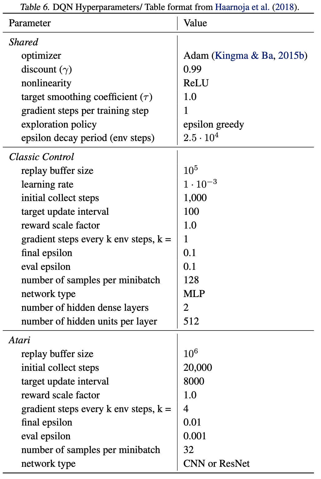
We investigate both value-based and policy-gradient methods. We chose DQN as the value-based algorithm, as it is the algorithm that first spurred the field of DRL, and has thus been extensively studied and extended. We chose two actor-critic algorithms for our investigations: an on-policy algorithm (PPO) and an off-policy one (SAC); both are generally considered to be state-of-the-art for many domains.
Environments
For discrete-control we focus on three classic control environments (CartPole, Acrobot, and MountainCar) as well as 15 games from the ALE Atari suite. For continuous-control we use five environments of varying difficulty from the MuJoCo suite (HalfCheetah, Hopper, Walker2d, Ant, and Humanoid).
Rewards obtained by DRL algorithms have notoriously high variance, so we repeat each experiment with at least 10 different seeds and report the average reward obtained over the last 10% of evaluations. We also provide 95% confidence intervals in all plots.
Training
For each sparse training algorithm considered (Pruning, Static, RigL, and SET) we train policies ranging between 50% to 99% sparsity. To ensure a fair comparison between algorithms, we performed a hyper parameter sweep for each algorithm separately. The exception is DQN experiments on Atari for which it was too computationally expensive to do a full hyper-parameter sweep and we used values found in previous experiments instead. Sparse results in these environments may therefore be conservative compared to the well tuned dense baseline. In addition to training the standard dense networks used in the literature, we also train smaller dense networks by scaling down layer widths to approximately match the parameter counts of the sparse networks, thereby providing a “parameter-equivalent” dense baseline.
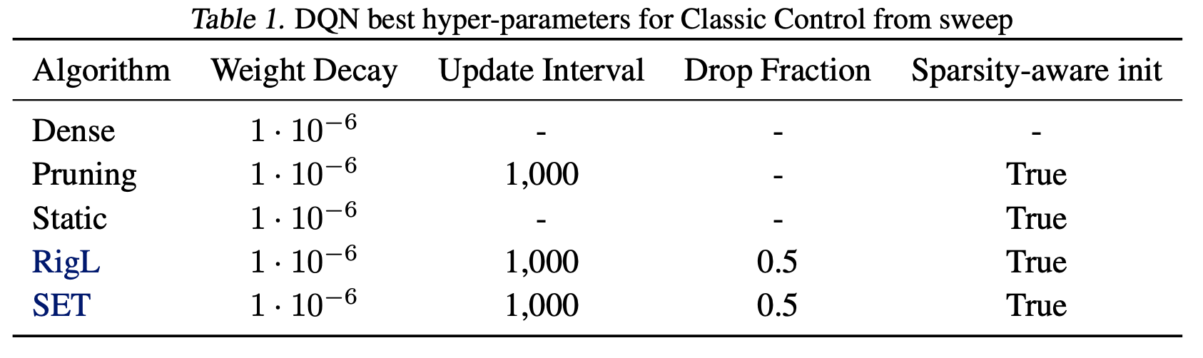
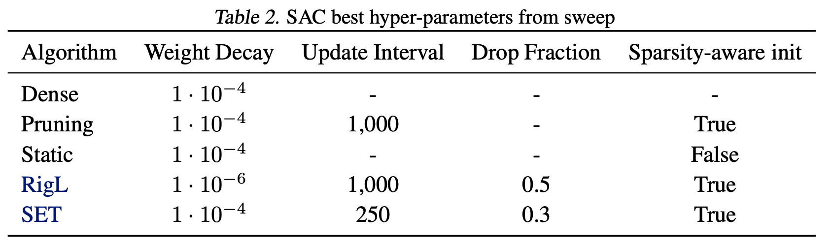
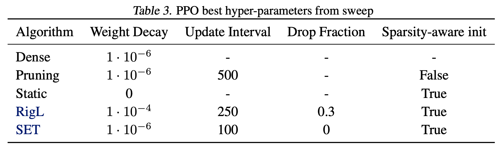
Hyper-parameter sweep details
We performed a grid search over different hyper parameters used in Dense, Prune, Static, SET and RigL algorithms. Unless otherwise noted, we use hyper-parameters used in regular dense training. When pruning, we start pruning around 20% of training steps and stop when 80% of training is completed following the findings of [Gale et al. (2019)](https://arxiv.org/abs/1902.09574). We use same default hyper-parameters for SET and RigL. Fort both algorithms we start updating the mask at initialization and decay the drop fraction over the course of the training using a cosine schedule, similar to pruning stopping the updates when 80% of training is completed.We searched over the following parameters:
- Weight decay: Searched over the grid [0, 1e-6, 1e-4, 1e-3].
- Update Interval: refers to how often models are pruned or sparse topology is updated. Searched over the grid [100, 250, 500, 1000, 5000].
- Drop fraction: refers to the maximum percentage of parameters that are dropped and added when network topology is updated. This maximum value is decayed during training according to a cosine decay schedule. Searched over the grid [0.0,0.1,0.2,0.3,0.5].
- Sparsity-aware initialization: refers to whether sparse models are initialized with scaled initialization or not.
We repeated the hyper-parameter search for each DRL algorithm using the Acrobot (for DQN) and Walker2D (for PPO and SAC) environments. Best hyper-parameters found in these environments are then used when training in other similar environments (i.e. classic control for DQN and MuJoCO for PPO and SAC). See the tables below for the best hyper parameters found in each setting.
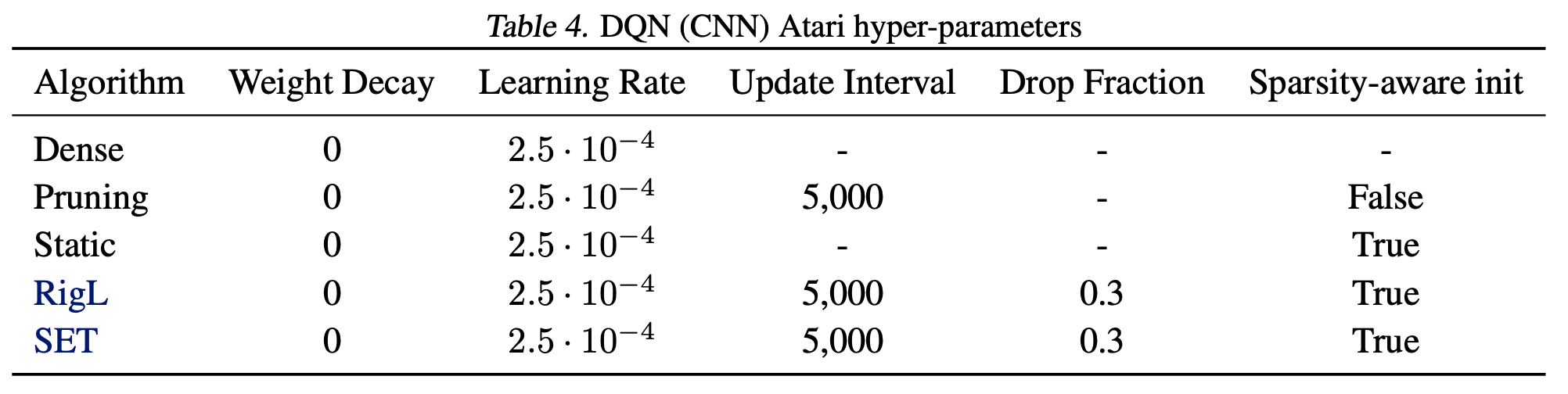
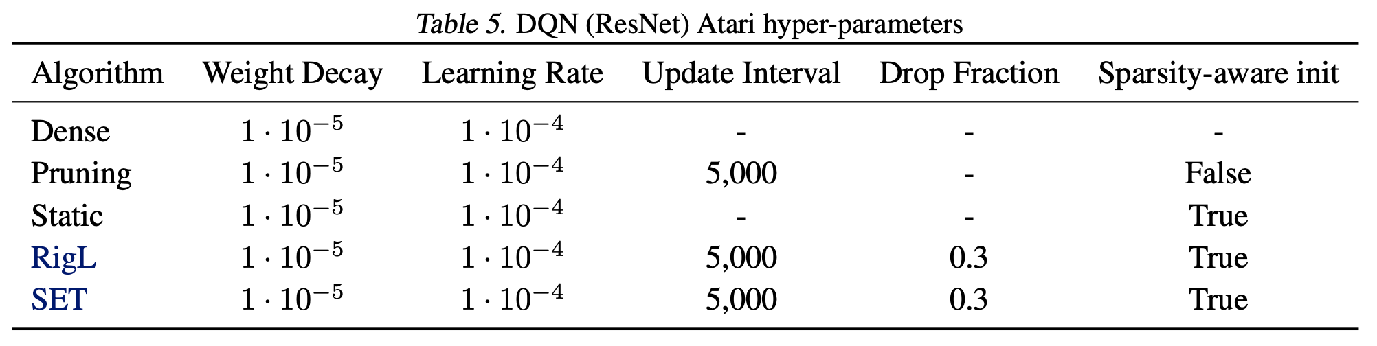
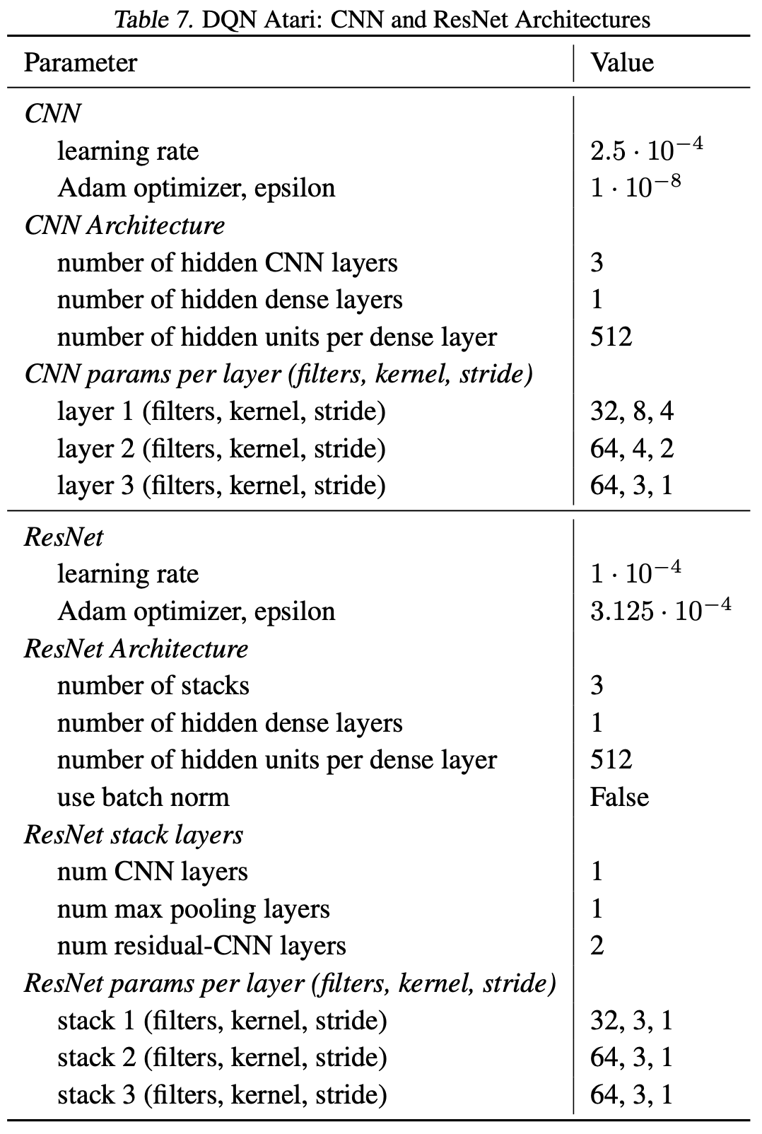
Atari hyper-parameters Due to computational constraints we did not search over hyper-parameters for the Atari environments, except for a small grid-search to tune the dense ResNet. The CNN architecture from Mnih et al. (2015) has been used in many prior works thus was already well tuned. The ResNet hyper-parameter sweep for the original dense model is detailed below:
- Weight decay: Searched over the grid [0, 1e-6, 1e-5, 1e-4]
- Learning rate: Searched over the grid [1e-4, 2.5e-4, 1e-3, 2.5e-3]
The final hyper-parameters we used for the Atari environments are shown in the two tables below for the CNN and ResNet architectures.
Remaining hyper-parameters Next, we include details of the DRL hyper-parameters used in all training settings.
Atari Game Selection
Our original three games (MsPacman, Pong, Qbert) were selected to have varying levels of difficulty as measured by DQN’s human normalized score in Mnih et al. (2015). To this we added 12 games (Assault, Asterix, BeamRider, Boxing, Breakout, CrazyClimber, DemonAttack, Enduro, FishingDerby, SpaceInvaders, Tutankham, VideoPinball) selected to be roughly evenly distributed amongst the games ranked by DQN’s human normalized score in Mnih et al. (2015) with a lower cut off of approximately 100% of human performance.
Code
Our code is available here, and is built upon the TF-Agents, Dopamine, and RigL codebases. We use rliable to calculate the interquantile mean (IQM) and plot the results.
The State of Sparse Networks in Deep RL
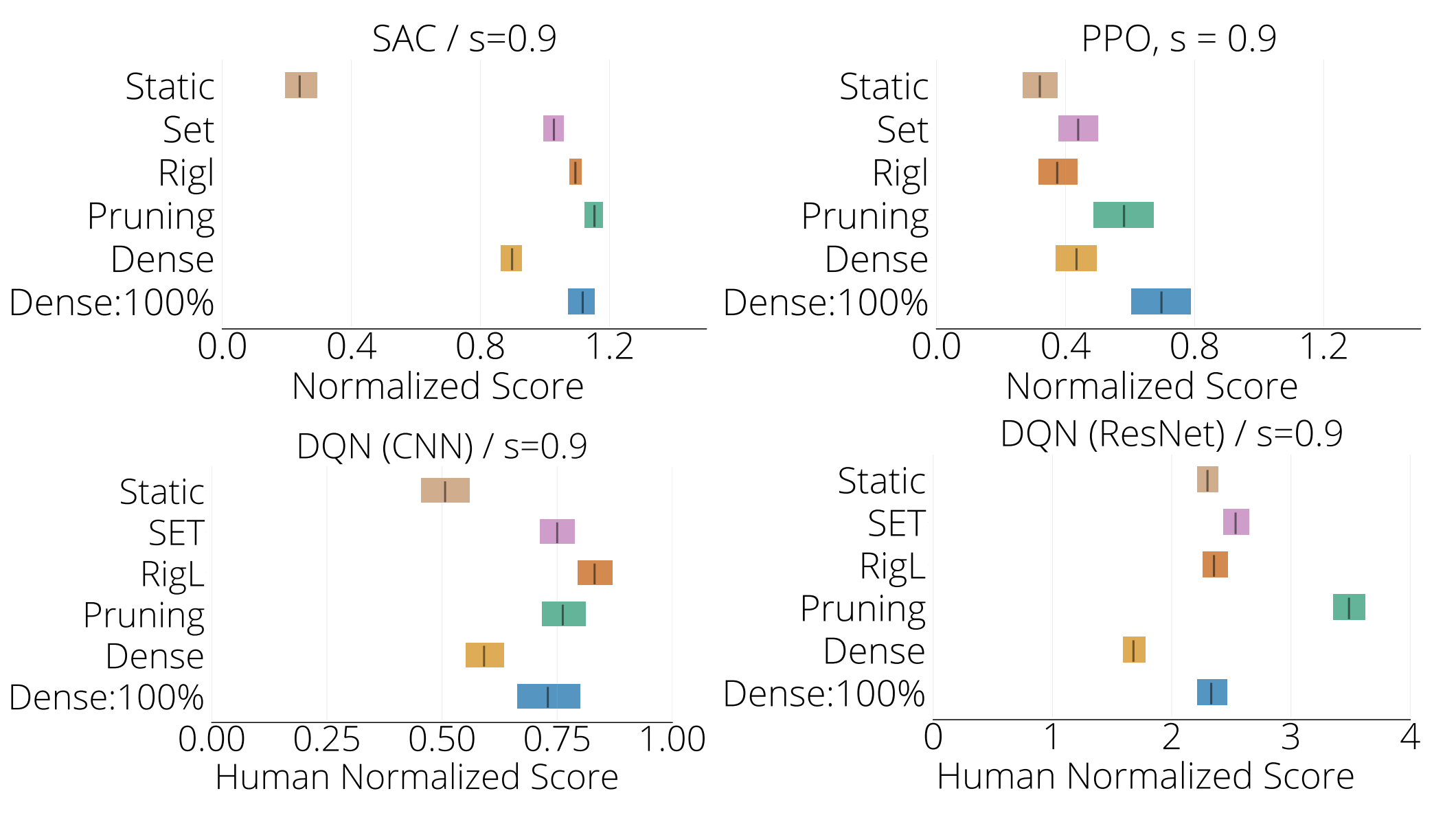
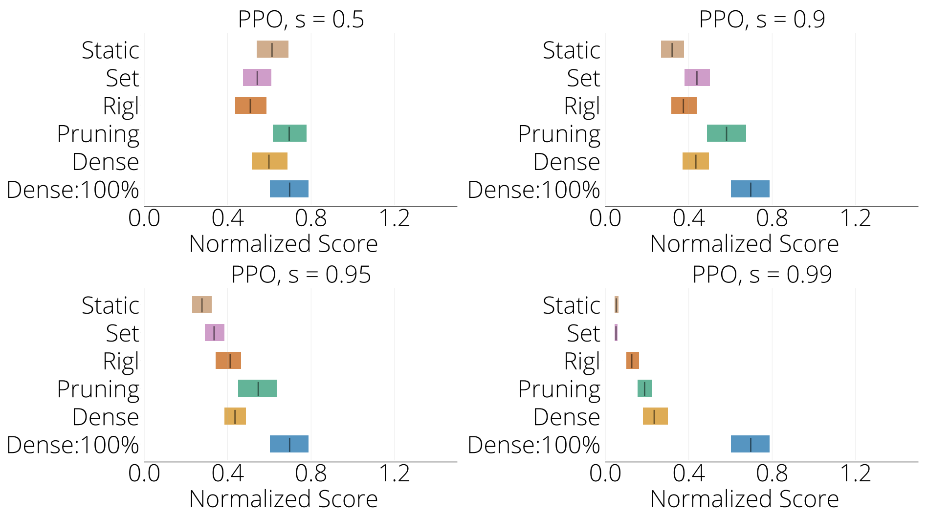
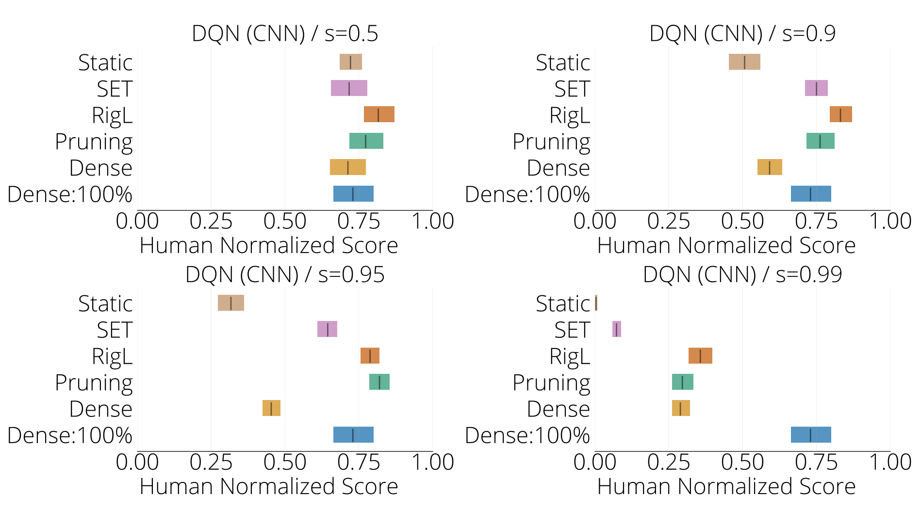
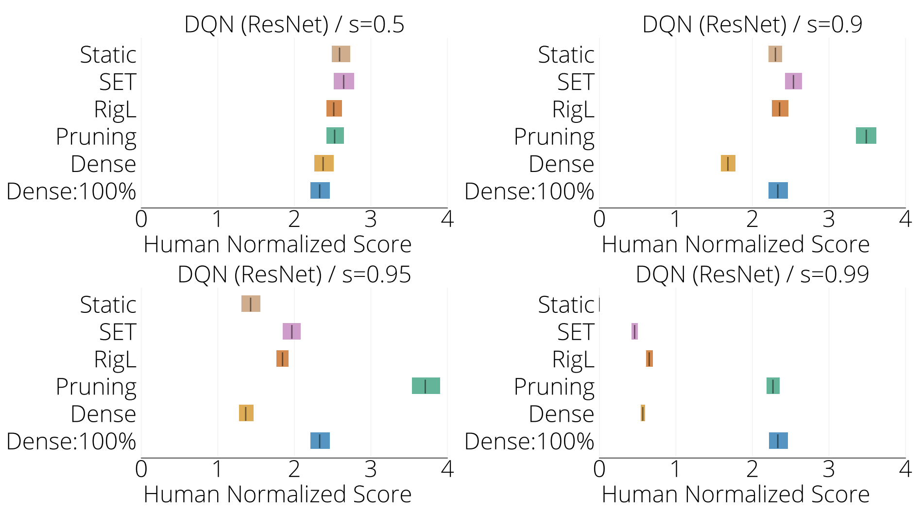
In the figure below we present the IQM at 90% sparsity for various architecture and algorithm combinations. SAC and PPO are averaged over 5 MuJoCo environments, whereas DQN is averaged over 15 Atari environments. “Dense: 100%” corresponds to the standard dense model. Atari scores were normalized using human performance per game. MuJoCo scores were normalized using the average returns obtained by the Dense: 100% SAC agent per game.
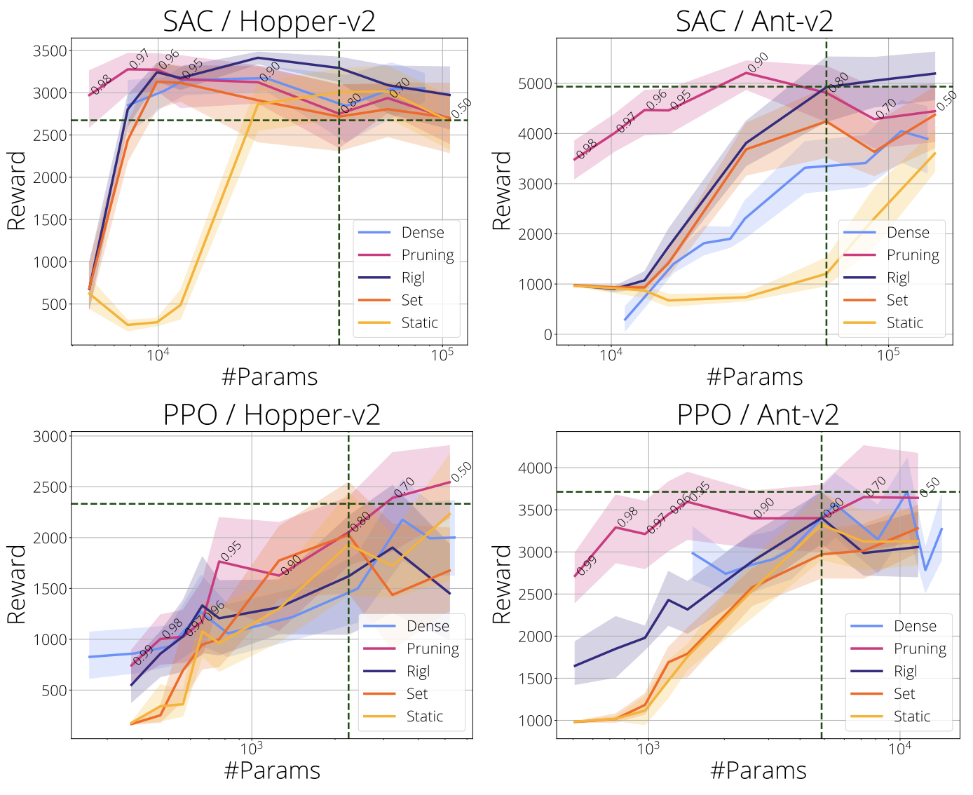
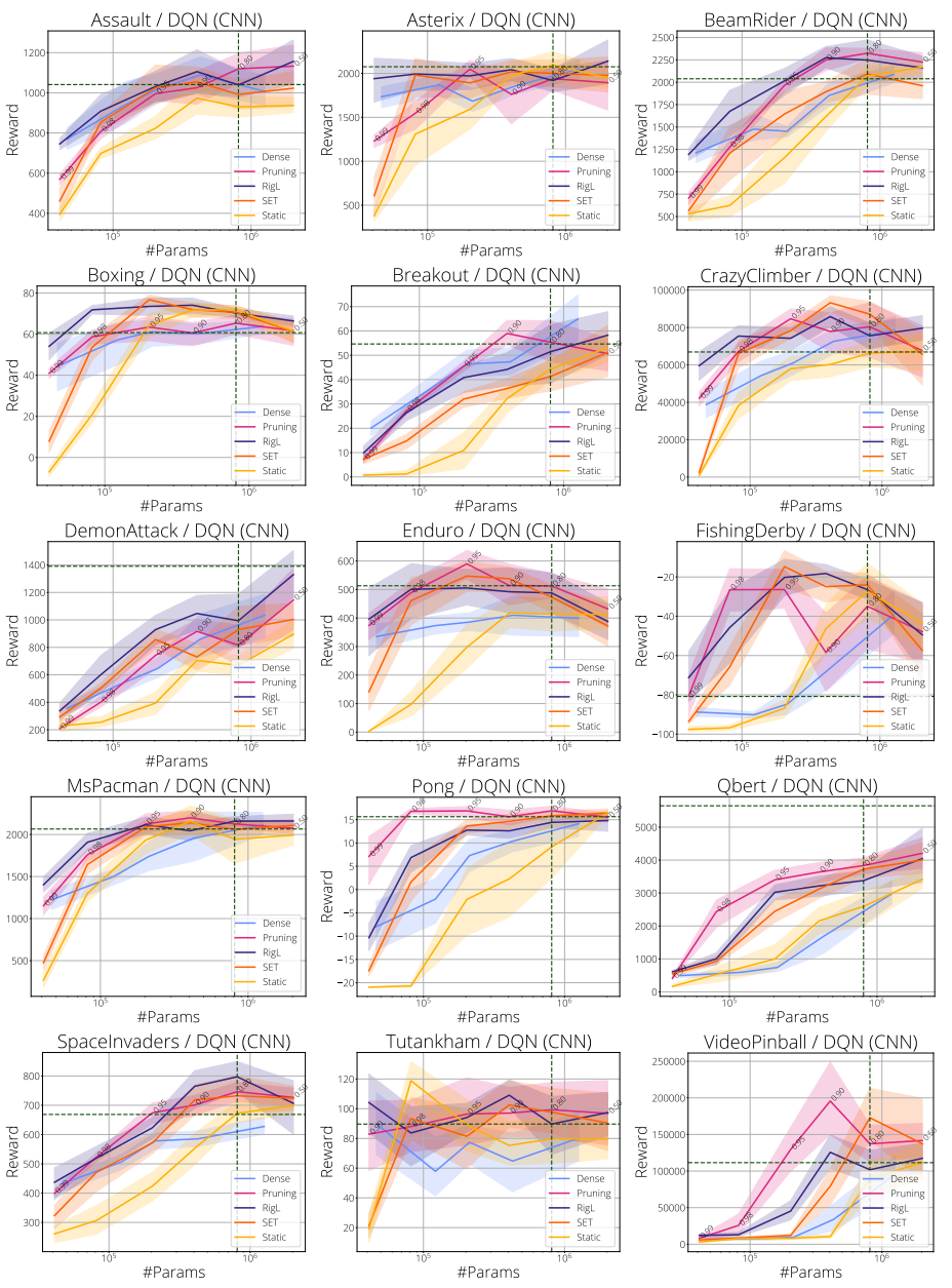
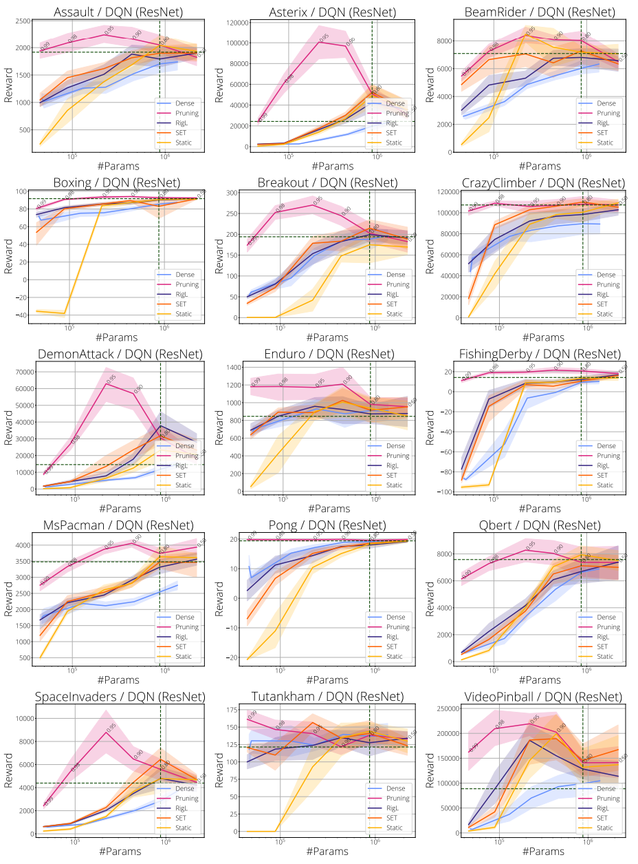
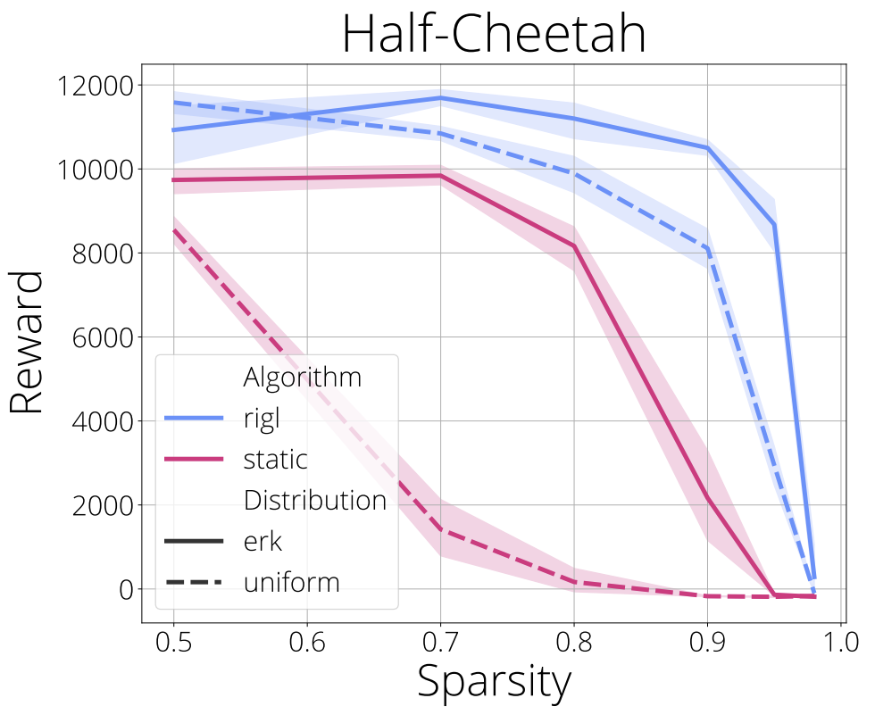
In the next figure we evaluate final performance relative to the number of parameters:
- (row-1) DQN on Atari (CNN)
- (row-2) SAC on MuJoCo
- (row-3) PPO on MuJoCo.
We consider sparsities from 50% to 95% (annotated on the pruning curve) for sparse training methods and pruning. Parameter count for networks with 80% sparsity and the reward obtained by the dense baseline are highlighted with vertical and horizontal lines. Shaded areas represent 95% confidence intervals.
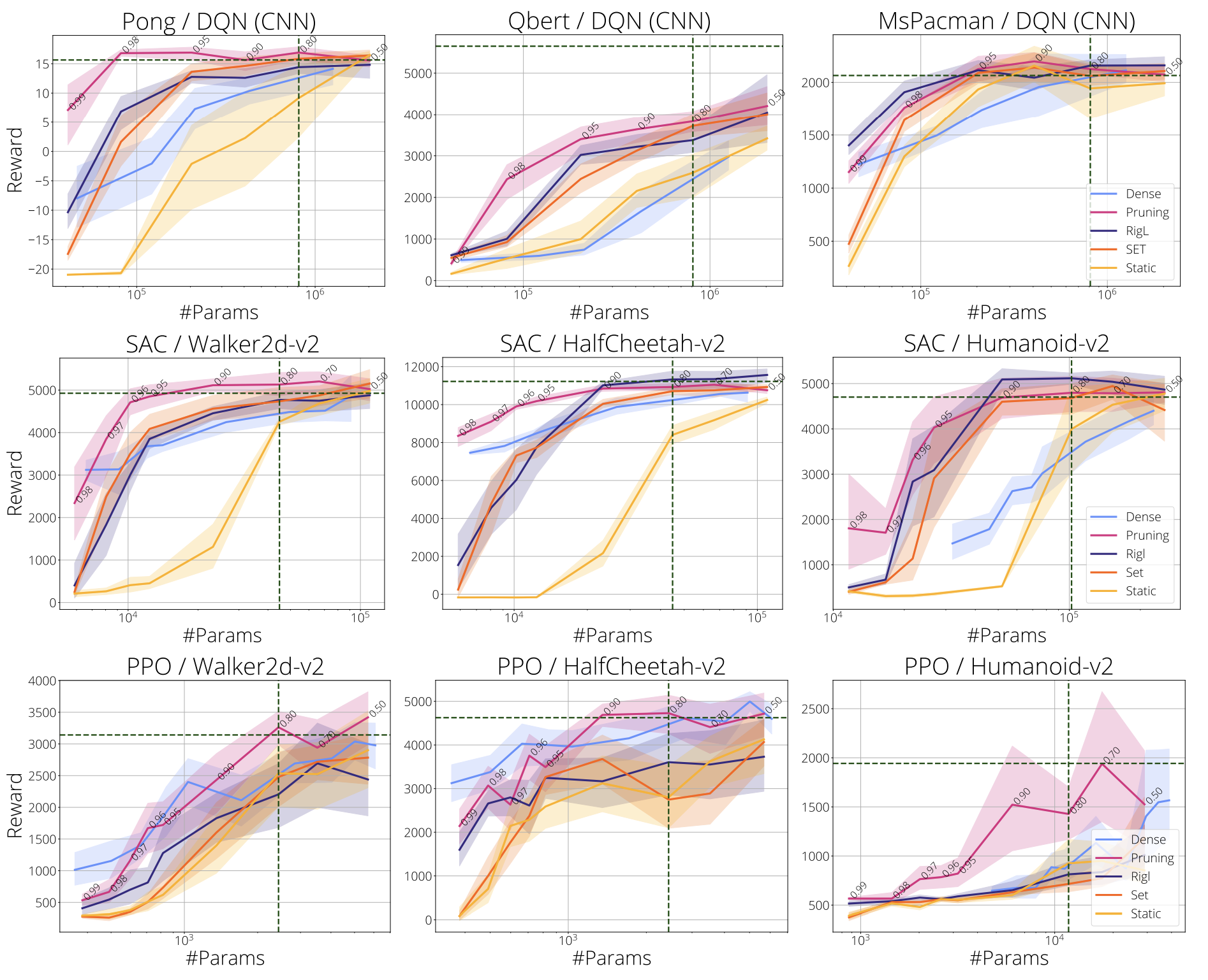
Three main conclusions emerge:
- In most cases performance obtained by sparse networks significantly exceeds that of their dense counterparts with a comparable number of parameters. Critically, in more difficult environments requiring larger networks (e.g. Humanoid, Atari), sparse networks can be obtained with efficient sparse training methods.
- It is possible to train sparse networks with up to 80-90% fewer parameters and without loss in performance compared to the standard dense model.
- Gradient based growing (i.e. RigL) seems to have limited impact on the performance of sparse networks.
More experimental results
In the figure below we compare final reward relative to parameter count using DQN on the classic control environments. ERK sparsity distribution was used in the top row whilst uniform was used in the bottom row.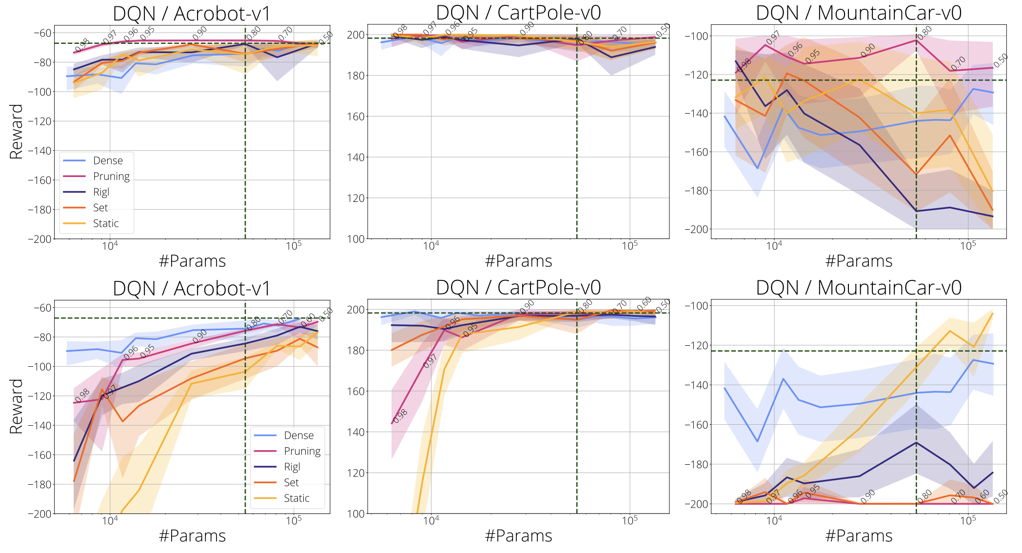
In the next figure we present results on the two remaining MuJoCo environment, Hopper and Ant with SAC (top row) and PPO (bottom row).
In the next two figures we show sparsity scaling plots for 15 Atari games using the standard CNN:
and for ResNet:
Additional IQM plots
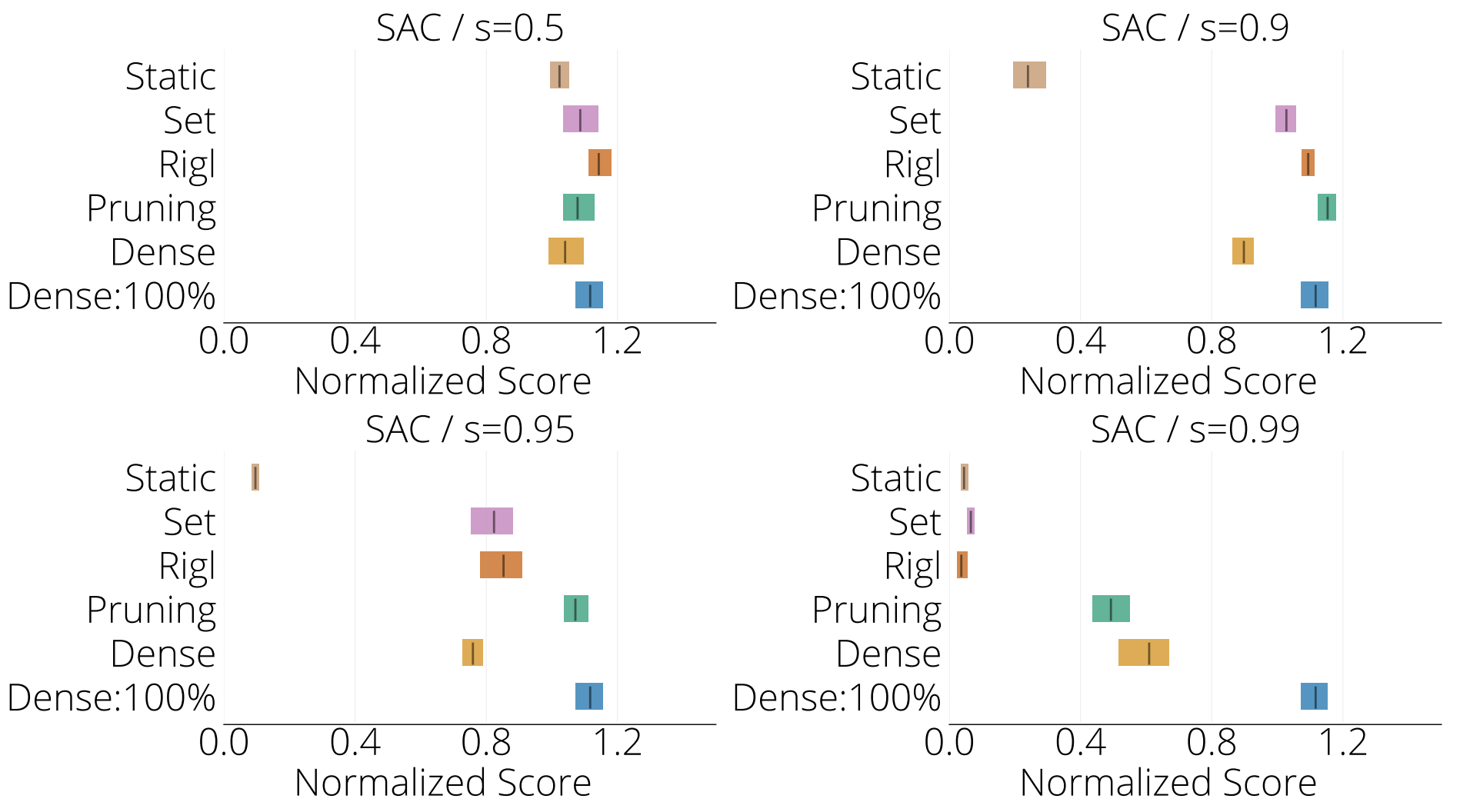
Mujoco SAC: In the figure below we present the interquartile mean (IQM) calculated over five Mujoco environments for SAC at four different sparsities, 50%, 90%, 95% and 99%, or the networks with the equivalent number of parameters in the case of Dense training. Note that for 99% sparsity the IQM is only calculated over three Mujoco environments.
Mujoco PPO: Next, we present the interquartile mean (IQM) calculated over five Mujoco environments for PPO at four different sparsities, 50%, 90%, 95% and 99%, or the networks with the equivalent number of parameters in the case of Dense training. Note that for 95% sparsity the IQM is calculated over four environments and for 99% sparsity the IQM is only calculated over three Mujoco environments.
Atari DQN: In the figure below we present IQM plots calculated over 15 Atari games for the standard CNN network architecture.
In the figure below we present IQM plots calculated over the same set of games for a ResNet architecture with an approximately equivalent number of parameters as the standard CNN (≈4M).
Next, we discuss each of these points in detail.
Sparse networks perform better
In line with previous observations made in speech, natural language modelling, and computer vision, in almost all environments, sparse networks found by pruning achieve significantly higher rewards than the dense baseline. However training these sparse networks from scratch (static) performs poorly. DST algorithms (RigL and SET) improve over static significantly, however often fall short of matching the pruning performance.
Critically, we observe that for more difficult environment requiring larger networks such as Humanoid, MsPacman, Qbert and Pong, sparse networks found by efficient DST algorithms exceed the performance of the dense baseline.
How sparse?
How much sparsity is possible without loss in performance relative to that of the standard dense model (denoted by Dense:100% in the first figure and by the horizontal lines in the second)?
We find that on average DST algorithms maintain performance up to 90% sparsity using SAC (Figure 1 top left) or DQN ( Figure 1 bottom row), after which performance drops. However performance is variable. For example, DST algorithms maintain performance especially well in MsPacman and Humanoid. Whereas in Qbert none of the methods are able to match the performance of the standard dense model at any of the examined levels of sparsity.
In the Atari environments, training a ResNet following the architecture from Espeholt et al. (2018) instead of the standard CNN alone provided about 3x improvement in IQM scores. We were also surprised to see that pruning at 90% sparsity exceeds the performance of the standard ResNet model.
These observations indicate that while sparse training can bring very significant efficiency gains in some environments, it is not a guaranteed benefit. Unlike supervised learning, expected gains likely depend on both task and network, and merits further inquiry.
RigL and SET
For most sparsities (50% - 95%) we observe little difference between these two sparse training algorithms. At very high sparsities, RigL may outperform SET. The difference can be large (e.g. MsPacman), but is more often moderate (e.g. Pong) or negligible (e.g. Humanoid, Qbert) with overlapping confidence intervals. This suggests that the gradient signal used by RigL may be less informative in the DRL setting compared to image classification, where it obtains state-of-the-art performance and consistently outperforms SET. Understanding this phenomenon could be a promising direction for improving sparse training methods for DRL.
Perhaps unsurprisingly, the clarity of the differences between sparse and dense training is affected by the stability of the underlying RL algorithm. Our results using SAC, designed for stability, were the clearest, as were the DQN results. In contrast, our results using PPO which has much higher variance, were less stark. For this reason, we used SAC and DQN when studying the different aspects of sparse agents in the rest of this work.
Where should sparsity be distributed?
When searching for efficient network architectures for DRL it is natural to ask where sparsity is best allocated. To that end, we consider both how to distribute parameters between network types and as well as within them.
Actor or Critic?
Although in value-based agents such as DQN there is a single network, in actor-critic methods such as PPO and SAC there are at least two: an actor and a critic network. It is believed that the underlying functions these networks approximate (e.g. a value function vs. a policy) may have significantly different levels of complexity, and this complexity likely varies across environments. Actor and critic typically have near-identical network architectures. However, for a given parameter budget it is not clear that this is the best strategy, as the complexity of the functions being approximated may vary significantly. We thus seek to understand how performance changes as the parameter ratio between the actor and critic is varied for a given parameter budget. In the following figure we assess three parameter budgets: 100%, 20% and 10% of the standard dense parameter count, and two training regimes, dense and sparse. Given the observed similarity in performance between RigL and SET we selected one method, RigL, for this analysis.
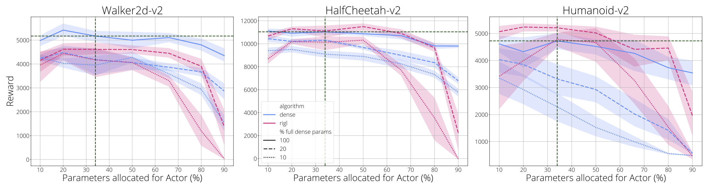
We observe that assigning a low proportion of parameters to the critic (10 - 20%) incurs a high performance cost across all regimes. When parameters are more scarce, in 20% and 10% of standard dense settings, performance degradation is highest. This effect is not symmetric. Reducing the actor parameters to just 10% rarely affects performance compared to the default actor-critic split of 34:66 (vertical line).
Interestingly the default split appears well tuned, achieving the best performance in most settings. However in the more challenging Humanoid environment we see that for smaller dense networks, reducing the actor parameters to just 10% yields the best performance. Sparse networks follow a similar trend, but we notice that they appear to be more sensitive to the parameter ratio, especially at higher sparsities.
Overall this suggests that the value function is the more complex function to approximate in these settings, benefiting from the lion’s share of parameters. It also suggests that tuning the parameter ratio may improve performance. Furthermore, FLOPs at evaluation time is determined only by the actor network. Since the actor appears to be easier to compress, this suggests large potential FLOPs savings for real-time usage of these agents. Finally, this approach could be used to better understand the relative complexity of policies and values functions across different environments.
Within network sparsity
In the figure below we turn our attention to the question of distributing parameters within networks and compare two strategies; uniform and ERK (Evci et al., 2020). Given a target sparsity of, say 90%, uniform achieves this by making each layer 90% sparse; ERK distributes them proportional to the sum of its dimension, which has the effect of making large layers relatively more sparse than the smaller ones. Due to weight sharing in convolutional layers, ERK sparsity distribution doubles the FLOPs required at a given sparsity, which we also found to be the case with the convolutional networks used by DQN in the Atari environments. On the other hand, ERK has no effect on the FLOPs count of fully connected networks used in MuJoCo environments.
Our results show that ERK significantly improves performance over uniform sparsity and thus we use ERK distribution in all of our experiments. We hypothesize the advantage of ERK is because it leaves input and output layers relatively more dense, since they typically have few incoming our outgoing connections, and this enables the network to make better use of (a) the observation and (b) the learned representations at the highest layers in the network. It is interesting to observe that maintaining a dense output layer is one of the key design decisions made by Sokar et al. (2021) for their proposed algorithm.
Sensitivity analysis
In this section we assess the sensitivity of some key hyperparameters for sparse training, and provide some findings for future research in this area.
Weight decay
In the figure below we evaluate the effect of weight decay and find that a small amount of weight decay is beneficial for pruning, RigL, and SET. This is to be expected since network topology choices are made based on weight magnitude, although we do note that the improvements are quite minor. Surprisingly weight decay seems to help dense even though it is not often used in DRL.
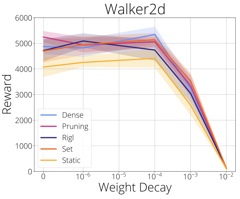
We recommend using small weight decay.
Sparsity-aware initialization
In the figure below we evaluate the effect of adjusting layer weight initialization based on a layer’s sparsity on static, RigL and SET. A common approach to initialization is to scale a weight’s initialization inversely by the square root of the number of incoming connections. Consequently, when we drop incoming connections, the initialization distribution should be scaled proportionately to the number of incoming connections (Evci et al., 2022). Our results show that this sparsity-aware initialization consistently improves performance when using uniform distribution over layer sparsities. However the difference disappears when using ERK for RigL and SET and may even harm performance for static.
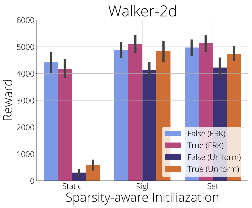
Performance is not sensitive to sparsity-aware initialization when using ERK and helps when using uniform layer sparsity. For RigL and SET we recommend always using sparsity-aware weight initialization (since it never appears to harm performance) but for static this may depend on layer sparsity.
Signal-to-noise ratio in DRL environments
Variance reduction is key to training deep models and often achieved through using momentum based optimizers. However when new connections are grown such averages are not available, therefore noise in the gradients can provide misleading signals. In the figure below we share the signal-to-noise ratio (SNR) for the Classic control and MuJoCo environments over the course of training. SNR is calculated as $\frac{|\mu|}{\sigma}$, where $\mu$ is the mean and $\sigma$ is the standard deviation of gradients over a mini-batch. A low SNR means the signal is dominated by the variance and thus the mean (the signal) is uninformative. We calculate SNR for all parameters separately and report the mean. Mini-batch gradients can have average SNR values as low as 0.01 starting early in training. Higher sparsities seem to cause lower SNR values. Similarly, actor networks have lower SNR.
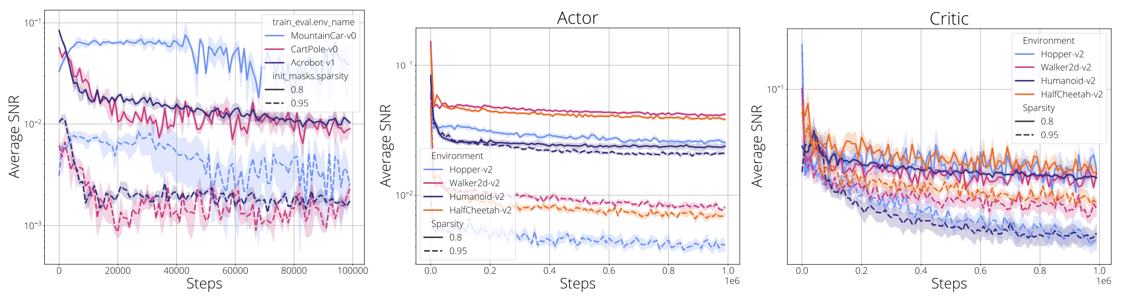
We find the average SNR for gradients to decrease with sparsity, potentially explaining the difficulty of using gradient based growing criteria in sparse training.
Are spare networks robust to noise?
Sparse neural networks can improve results on primary metrics such accuracy and rewards, yet they might have some unexpected behaviours in other aspects. In the figure below we assess the effect of adding increasing amounts of noise to the observations and measuring their effect on a trained policy. Noise was sampled $\sim\mathcal{N}(0, \sigma)$, $\sigma\in [0, 1, \ldots, 30]$, quantized to an integer, and added to each observation’s pixel values ($\in [0, 255]$) before normalization. Noise was sampled independently per pixel. We look at three data regimes; 100%, 50% and 10% of the standard dense model parameter count and compare dense and sparse training (RigL and SET). We made an effort to select policies with comparable performance for all the methods, chosen from the set of all policies trained during this work.
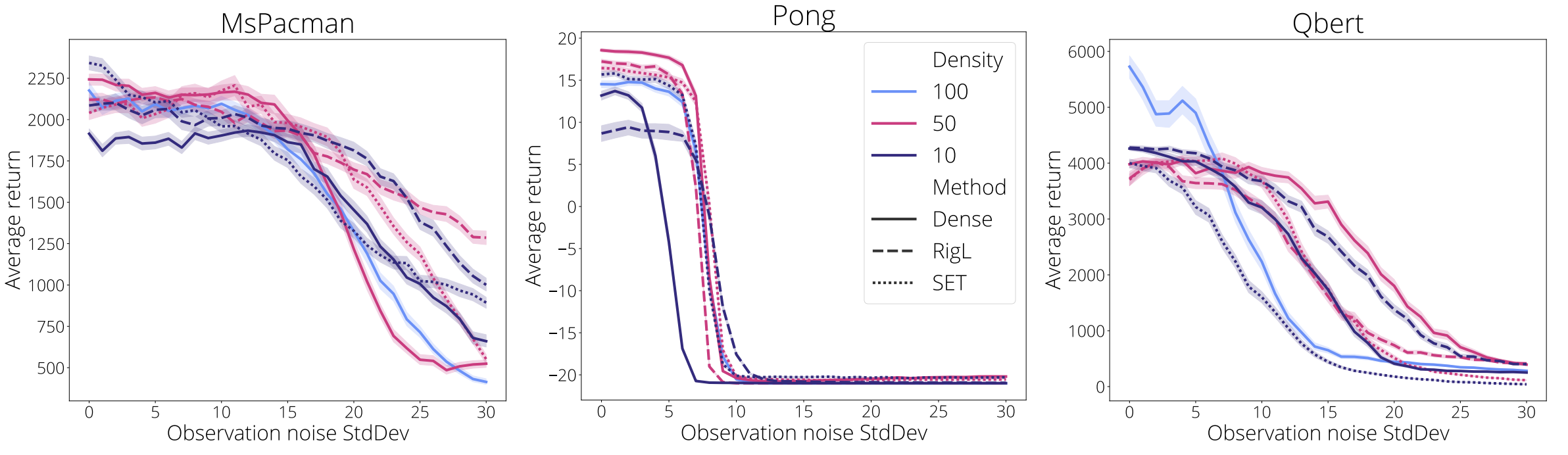
We observe that
- Smaller models are generally more robust to high noise than larger models
- Sparse models are more robust to high noise than dense models on average
- In most cases there are minimal differences when the noise is low.
We can see that in the very low data regime (10% full parameter count) policies trained using RigL are more robust to high noise compared with their dense counterparts, a fact observed across every environment. In the moderate data regime (50% full parameter count) the ordering is more mixed. In Qbert the dense model is most robust but the picture is reversed for Pong and McPacman. Finally, SET appears less robust to high noise than RigL, although we note this is not the case for Pong at 50% density.
Although a preliminary analysis, it does suggest that sparse training can produce networks that are more robust to observational noise, even when experienced post-training.
Discussion and Conclusion
In this work we sought to understand the state of sparse training for DRL by applying pruning, static, SET and RigL to DQN, PPO, and SAC agents trained on a variety of environments. We found sparse training methods to be a drop-in alternative for their dense counterparts providing better results for the same parameter count. From a practical standpoint we made recommendations regarding hyper-parameter settings and showed that non-uniform sparse initialization combined with tuning actor:critic parameter ratios improves performance. We hope this work establishes a useful foundation for future research into sparse DRL algorithms and highlights a number of interesting research questions. In contrast to the computer vision domain, we observe that RigL fails to match pruning results. Low SNR in high sparsity regimes offers a clue but more work is needed to understand this phenomena. Our results evaluating robustness to noise also suggest that sparse networks may aid in generalization and robustness to observational noise; this is an active area of interest and research in the DRL community, so a more thorough understanding could result in important algorithmic advances.
Acknowledgements
The authors would like to thank Fabian Pedregosa, Rishabh Agarwal, and Adrien Ali Ta¨ıga for their helpful feedback on the manuscript, Oscar Ramirez for his help with on the TF-Agents codebase, and Trevor Gale and Sara Hooker for inspiring the title of this work. We also thank Brain Montreal RL team for their useful feedback on an early version of this work. Finally, we thank Bram Grooten for pointing out Degrave et al. (2022) and their contribution to the motivation for this work.
comments powered by Disqus