Scalable methods for computing state similarity in deterministic MDPs

This post describes my paper Scalable methods for computing state similarity in deterministic MDPs, published at AAAI 2020. The code is available here.

Motivation

We consider distance metrics between states in an MDP. Take the following MDP, where the goal is to reach the green cells:

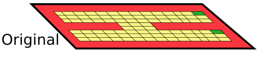
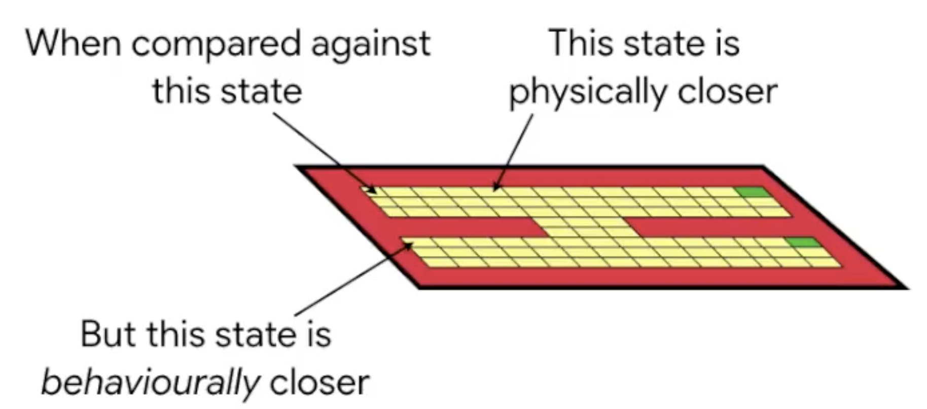
Physical distance betweent states?

Physical distance often fails to capture the similarity properties we’d like:

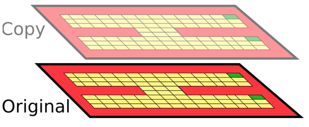
State abstractions

Now imagine we add an exact copy of these states to the MDP (think of it as an additional “floor”):

And imagine after each action the agent randomly transitions between these two floors:

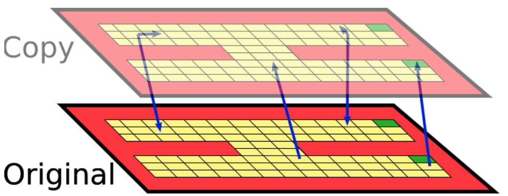
Notice that since the optimal policy is identical on both floors, we just doubled the state space for no reason! We should really be grouping together similar states.

MDPs

Consider the standard MDP defintion $\langle\mathcal{S}, \mathcal{A}, \mathcal{R}, \mathcal{P}, \gamma\rangle$, where $\mathcal{S}$ is the state space, $\mathcal{A}$ is the action space, $\mathcal{R}:\mathcal{S}\times\mathcal{A}\rightarrow\mathbb{R}$ is the one-step reward function, $\mathcal{P}:\mathcal{S}\times\mathcal{A}\rightarrow\Delta(\mathcal{S})$ is the next-state distribution function, and $\gamma\in [0, 1)$ is the discount factor.

Bisimulation

What we need is a notion of state distance that captures behavioural indistinguishability.

Equivalence relations

First, let me explain bisimulation relations, which was introduced by Givan, Dean, and Greig.

Two states, $s$ and $t$, are considered bisimlar (denoted $s\sim t$) if, under all actions:

1. They have equal immediate rewards: $$ \forall a\in\mathcal{A}.\quad \mathcal{R}(s, a) = \mathcal{R}(t, a) $$
2. Transition with equal probability to bisimulation equivalence classes: $$ \forall a\in\mathcal{A}, \forall c\in\mathcal{S}/_{\sim}.\quad\mathcal{P}(s, a)(c) := \sum_{s’\in c}\mathcal{P}(s, a)(s’) = \mathcal{P}(t, a)(c)$$

This is often easiest to understand via an illustration. Consider the folloowing system:

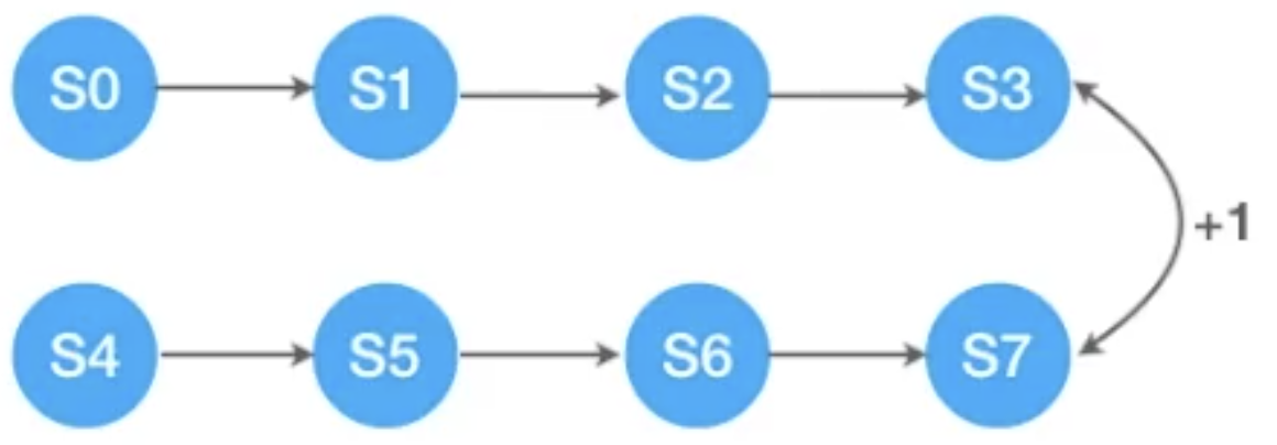
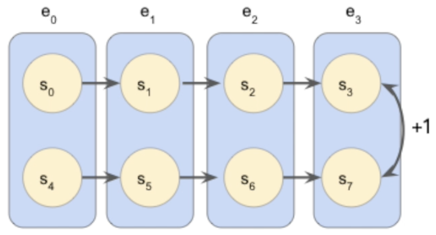
A bisimulation equivalence relation would collapse the 8 states above into an equivalent 4-state MDP:

But, unfortunately, bisimulation equivalence is brittle, as it’s a 0/1 relationship!

Metrics

Bisimulation metrics generalize bisimulation relations, and quantify the behavioural distance between two states in an MDP. They are defined as any metric $d$ where $d(s, t) = 0 \iff s\sim t$. Ferns, Panangaden, and Precup proved that the following operator admits a fixed point $d^{\sim}$, and this fixed point is a bisimulation metric:

$$ F(d)(s, t) = \max_{a\in\mathcal{A}}\left[ |R(s, a) - R(t, a)| + \gamma T_K(d)(P(s, a), P(t, a)) \right] $$

where $s,t\in\mathcal{S}$ are two states in the MDP, $\mathcal{A}$ is the action space, $R:\mathcal{S}\times\mathcal{A}\rightarrow\mathbb{R}$ is the reward function, $P:\mathcal{S}\times\mathcal{A}\rightarrow\Delta(\mathcal{S})$ is the transition function, and $T_K(d)$ is the Kantorovich (also known as the Wasserstein, Earth Mover’s, Sinkhorn, …) distance between two probability distributions under a state metric $d$.

These metrics have nice theoretical properties, such as: the bisimulation distance between two states is an upper-bound on their optimal value difference:

Shortcomings and solutions

Bisimulation metrics have three shortcomings I address in my paper.

Pessimism

Problem

They’re inherently pessimistic (the max is considering the worst possible case!): $$ F(d)(s, t) = {\color{red} \max_{a\in\mathcal{A}}}\left[ |R(s, a) - R(t, a)| + \gamma T_K(d)(P(s, a), P(t, a)) \right] $$ Take the following example MDP, where edge labels indicate the action (${a, b}$) and non-zero rewards ($[K]$).

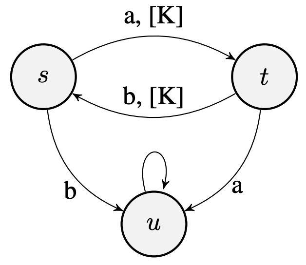
When $\gamma = 0.9$, $V^∗(s) = V^∗(t) = 10K$, while $d^{\sim}(s, t) = 10K$, which shows that the bound mentioned in the last section can be made to be as loose as desired.

Solution

I introduce on-policy bisimulation metrics, $d^{\pi}_{\sim}$. These are similar to regular bisimulation metrics, but are defined with respect to a policy $\pi:\mathcal{S}\rightarrow\Delta(\mathcal{A})$. In the paper I prove that $$ |V^{\pi}(s) - V^{\pi}(t) | \leq d^{\pi}_{\sim}(s, t) $$

Computational Expense

Problem

Bisimulation metrics have been traditionally solved via dynamic programming. But this can be very expensive, as it requires updating the metric estimate for all state-action pairs at every iteration! Note that this means computing the Kantorovich (which is an expensive linear program) $|\mathcal{S}|\times|\mathcal{A}|$ times at each iteration.

Solution

Sampling! If we assume a deterministic MDP, I provide an update rule using sampled pairs of $\langle s, a, r, s’\rangle$ transitions, and prove that this is guaranteed to converge to the true metric! See Theorem 4 in the paper for details.

Full state enumerability

Problem

Existing methods for computing/approximating bisimulation metrics require full state enumerability.

Solution

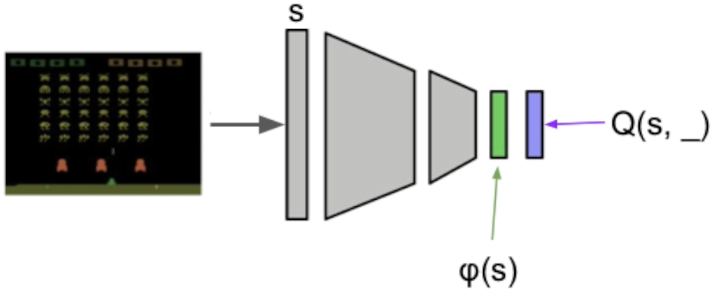
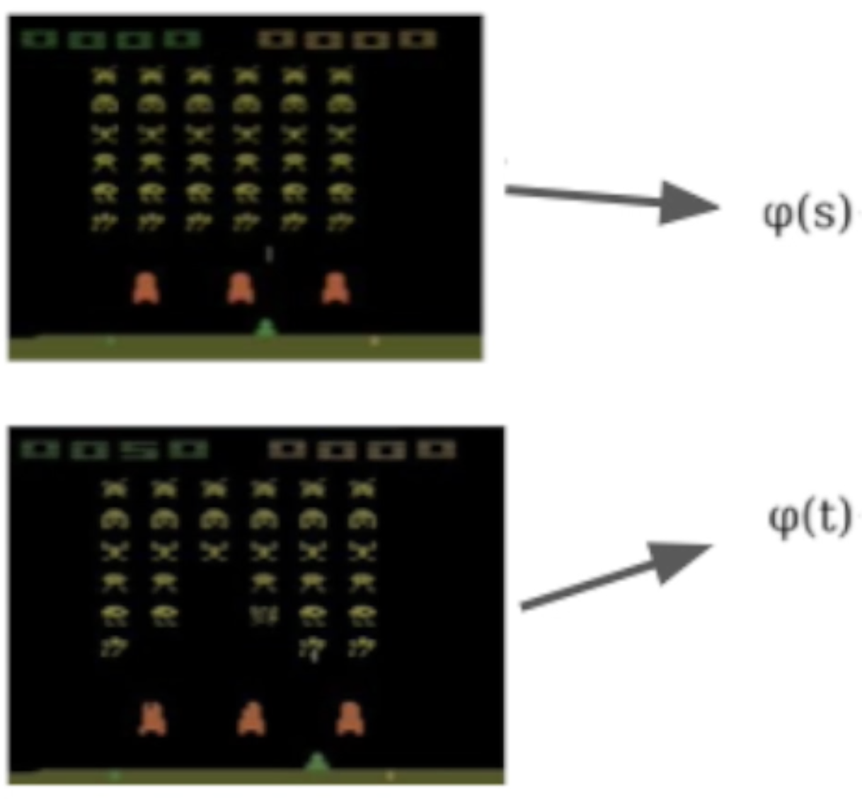
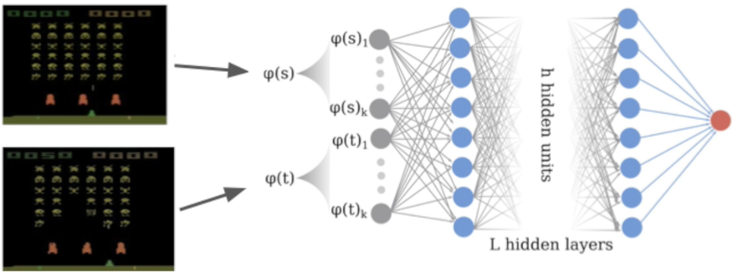
Use neural networks! Consider a trained Rainbow agent, and take the penultimate layer as the representation ($\phi$):

We can concatenate the representations of two states:

And feed them through a neural network, where we denote the output of the network as $\psi(s, t)$:

We define a target for regular bisimulation ($s’$ and $t’$ are the unique next states from $s$ and $t$, respectively): $$ \mathbf{T}_{\theta}(s, t, a) = \max (\psi_{\theta}(s, t, a), |\mathcal{R}(s, a)-\mathcal{R}(t, a)| + \gamma\psi_{\theta}(s’, t’))$$

and for on-policy bisimulation: $$ \mathbf{T}^{\pi}_{\theta}(s, t, a) = |\mathcal{R}^{\pi}(s)-\mathcal{R}^{\pi}(t)| + \gamma\psi^{\pi}_{\theta}(s’, t’))$$

Which is then incorporated into the loss (where $\mathcal{D}$ is the dataset, e.g. a replay buffer): $$ \mathcal{L}^{(\pi)}_{s,t,a} = \mathbb{E}_{\mathcal{D}}\left(\mathbf{T}^{(\pi)}_{\theta}(s, t, a) - \psi^{(\pi)}_{\theta}(s, t, a)\right)^2 $$

Evaluate on Atari 2600

Take a trained Rainbow agent and compute the distance from the first state:

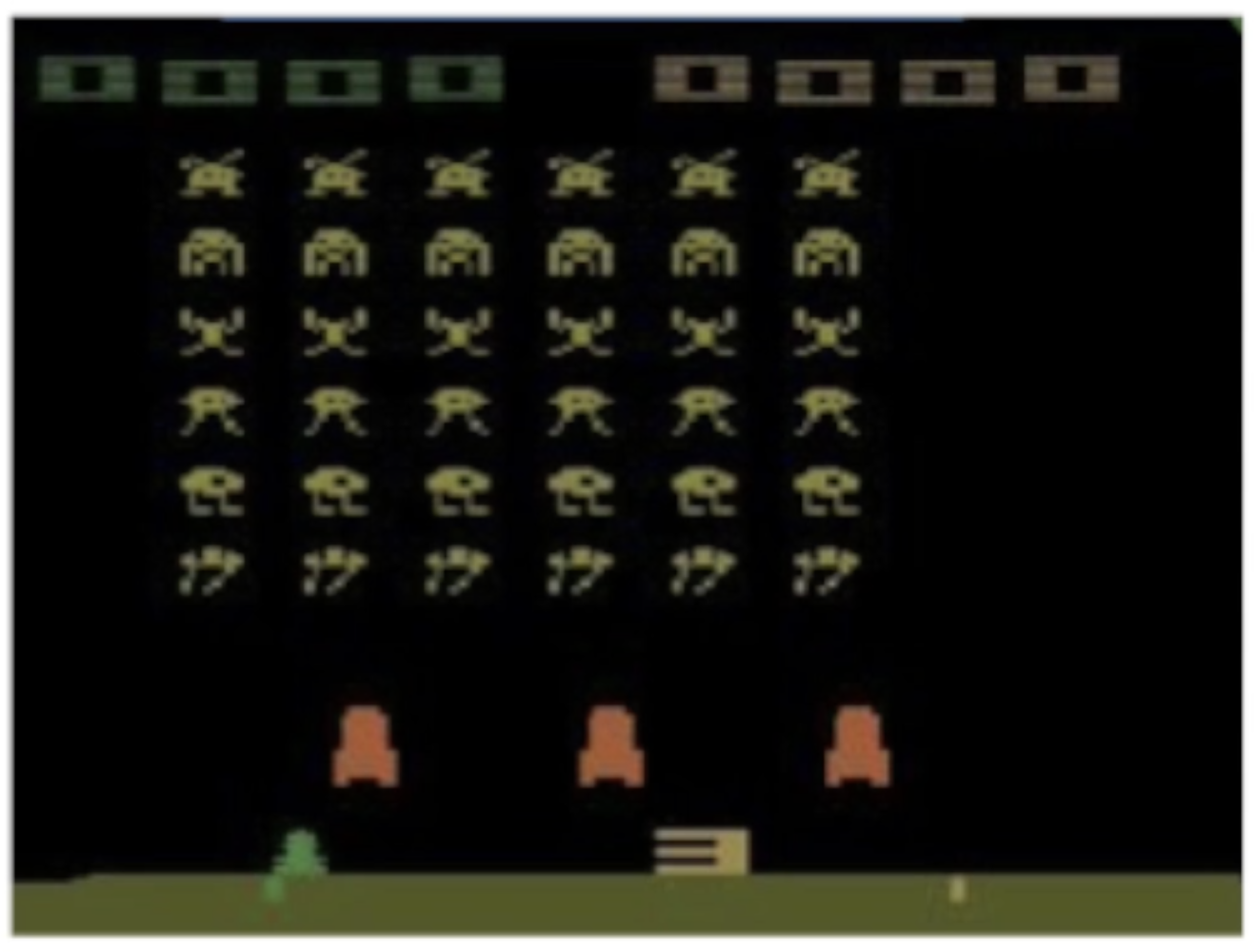
to every other state:

Let’s see the results! Notice how the metric jumps when an alien ship is destroyed:

Citing

The original tweet is here.

Please use the following BibTeX entry if you’d like to cite this work:

@inproceedings{castro20bisimulation,
  author    = {Pablo Samuel Castro},
  title     = {Scalable methods for computing state similarity in deterministic {M}arkov {D}ecision {P}rocesses},
  year      = {2020},
  booktitle = {Proceedings of the Thirty-Fourth AAAI Conference on Artificial Intelligence (AAAI-20)},
}