
Pablo Samuel Castro
December 6, 2021
Deep Reinforcement Learning at the Edge of the Statistical Precipice
We argue that reliable evaluation in the few run deep RL regime cannot ignore the uncertainty in results without running the risk of slowing down progress in the field. We illustrate this point using a case study on the Atari 100k benchmark, where we find substantial discrepancies between conclusions drawn from point estimates alone versus a more thorough statistical analysis. We advocate for reporting interval estimates of aggregate performance and propose performance profiles to account for the variability in results, as well as present more robust and efficient aggregate metrics, such as interquartile mean scores, to achieve small uncertainty in results.
Rishabh Agarwal, Max Schwarzer, Pablo Samuel Castro, Aaron Courville, and Marc G. Bellemare
This blogpost is a summary of our NeurIPS 2021 paper (winner of an outstanding paper award). The code is available here.
Introduction
Research in artificial intelligence, and particularly deep reinforcement learning (RL), relies on evaluating aggregate performance on a diverse suite of tasks to assess progress. Quantitative evaluation on a suite of tasks, such as Atari games, reveals strengths and limitations of methods while simultaneously guiding researchers towards methods with promising results. Performance of RL algorithms is usually summarized with a point estimate of task performance measure, such as mean and median performance across tasks, aggregated over independent training runs.
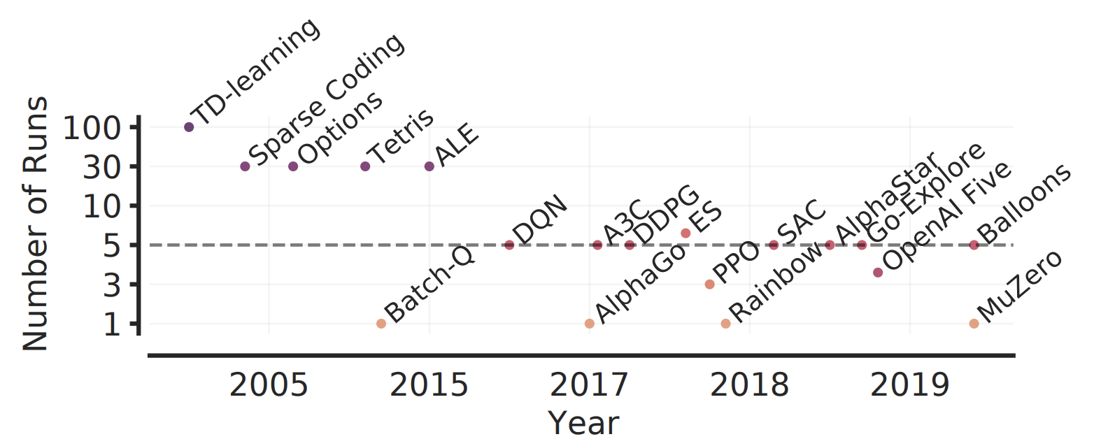
A small number of training runs coupled with high variability in performance of deep RL algorithms, often leads to substantial statistical uncertainty in reported point estimates. While evaluating more runs per task has been prescribed to reduce uncertainty and obtain reliable estimates, 3-10 runs are prevalent in deep RL as it is often computationally prohibitive to evaluate more runs. For example, 5 runs each on 50+ Atari 2600 games in ALE using standard protocol requires more than 1000 GPU training days. As we move towards more challenging and complex RL benchmarks (e.g., StarCraft), evaluating more than a handful of runs will become increasingly demanding due to increased amount of compute and data needed to tackle such tasks. Additional confounding factors, such as exploration in the low-data regime, exacerbates the performance variability in deep RL – as seen on the Atari 100k benchmark – often requiring many more runs to achieve negligible statistical uncertainty in reported estimates.
Ignoring the statistical uncertainty in deep RL results gives a false impression of fast scientific progress in the field. It inevitably evades the question: “Would similar findings be obtained with new independent runs under different random conditions?” This could steer researchers towards superficially beneficial methods, often at the expense of better methods being neglected or even rejected early as such methods fail to outperform inferior methods simply due to less favorable random conditions. Furthermore, reporting point estimates can erroneously lead the field to conclude which methods are state-of-the-art, ensuing wasted effort and sometimes degradation in performance over existing methods when applied in practice. Moreover, not reporting the uncertainty in deep RL results makes them difficult to reproduce except under the exact same random conditions, which could lead to a reproducibility crisis similar to the one that plagues other fields. Finally, unreliable results could erode trust in deep RL research itself.
In this work, we show that recent deep RL papers compare unreliable point estimates, which are dominated by statistical uncertainty, as well as exploit non-standard evaluation protocols, using a case study on Atari 100k. Then, we illustrate how to reliably evaluate performance with only a handful of runs using a more rigorous evaluation methodology that accounts for uncertainty in results. To exemplify the necessity of such methodology, we scrutinize performance evaluations of existing algorithms on widely used benchmarks, including the ALE (Atari 100k, Atari 200M), Procgen and DeepMind Control Suite, again revealing discrepancies in prior comparisons. Our findings call for a change in how we evaluate performance in deep RL, for which we present a better methodology to prevent unreliable results from stagnating the field.
How do we reliably evaluate performance on deep RL benchmarks with only a handful of runs? As a practical solution that is easily applicable with 3-10 runs per task, we identify three statistical tools for improving the quality of experimental reporting (see Table below). Since any performance estimate based on a finite number of runs is a random variable, we argue that it should be treated as such. Specifically, we argue for reporting aggregate performance measures using interval estimates via stratified bootstrap confidence intervals, as opposed to point estimates. Among prevalent aggregate measures, mean can be easily dominated by performance on a few outlier tasks, while median has high variability and zero performance on nearly half of the tasks does not change it. To address these deficiencies, we present more efficient and robust alternatives, such as interquartile mean, which are not unduly affected by outliers and have small uncertainty even with a handful of runs. Furthermore, to reveal the variability in performance across tasks, we propose reporting performance distributions across all runs. Compared to prior work, these distributions result in performance profiles that are statistically unbiased, more robust to outliers, and require fewer runs for smaller uncertainty.
| Desideratum | Current Evaluation Protocol | Our Recommendation |
|---|---|---|
| Uncertainty in aggregate performance | Point estimates - Ignore statistical uncertainty - Hinder results reproducibility | Interval estimates via stratified bootstrap confidence intervals |
| Variability in performance across tasks and runs | Tables with mean scores per task«br> - Overwhelming beyond a few tasks - Standard deviations often omitted - Incomplete picture for multimodal and heavy-tailed distributions | Performance profiles (score distributions) - Show tail distribution of scores on combined runs across tasks - Allow qualitative comparisons - Easily read any score percentile |
| Aggregate metrics for summarizing performance across tasks | Mean - Often dominated by performance on outlier tasks Median - Requires large number of runs to claim improvements - Poor indicator of overall performance: zero scores on nearly half the tasks do not affect it | Interquartile Mean (IQM) across all runs - Performance on middle 50% of combined runs - Robust to outlier scores but more statistically efficient than median To show other aspects of performance gains, report average probability of improvement and optimality gap. |
Formalism
We consider the setting in which a reinforcement learning algorithm is evaluated on $M$ tasks. For each of these tasks, we perform $N$ independent runs (A run can be different from using a fixed random seed. Indeed, fixing the seed may not be able to control all sources of randomness such as non-determinism of ML frameworks with GPUs) which each provide a scalar, normalized score $x_{m,n}$, $m=1,\ldots ,M$ and $n=1,\ldots ,N$. These normalized scores are obtained by linearly rescaling per-task scores based on two reference points; for example, performance on the Atari games is typically normalized with respect to a random agent and an average human, who are assigned a normalized score of 0 and 1 respectively. We denote the set of normalized scores by $x_{1:M,1:N}$.
In most experiments, there is inherent randomness in the scores obtained from different runs. This randomness can arise from stochasticity in the task, exploratory choices made during learning, randomized initial parameters, but also software and hardware considerations such as non-determinism in GPUs and in machine learning frameworks. Thus, we model the algorithm’s normalized score on the $m^{th}$ task as a real-valued random variable $X_{m}$. Then, the score $x_{m, n}$ is a realization of the random variable $X_{m,n}$, which is identically distributed as $X_{m}$. For $\tau \in \mathbb{R}$, we define the tail distribution function of $X_m$ as $F_m(\tau) = \Pr(X_m > \tau)$. For any collection of scores $y_{1:K}$, the empirical tail distribution function is given by $\hat F(\tau; y_{1:K}) = \tfrac{1}{K} \sum_{k=1}^{K} \mathbb{1}[y_k > \tau]$. In particular, we write $\hat{F}_m(\tau) = \hat F(\tau; x_{m, 1:N})$.
The aggregate performance of an algorithm maps the set of normalized scores $x_{{1:M}, {1:N}}$ to a scalar value. Two prevalent aggregate performance metrics are the mean and median normalized scores. If we denote by $\bar{x}_m = \tfrac{1}{N} \sum_{n=1}^N x_{m,n}$ the average score on task $m$ across $N$ runs, then these aggregate metrics are $\text{Mean}({\bar x}_{1:M})$ and $\text{Median}({\bar x}_{1:M})$. More precisely, we call these sample mean and sample median over the task means since they are computed from a finite set of $N$ runs. Since $\bar{x}_m$ is a realization of the random variable $\bar{X}_m = \tfrac{1}{N} \sum_{n=1}^N X_{m,n}$, the sample mean and median scores are point estimates of the random variables $\text{Mean}({\bar X}_{1:M})$ and $\text{Median}({\bar X}_{1:M})$ respectively. We call true mean and true median the metrics that would be obtained if we had unlimited experimental capacity ($N \to \infty$), given by $\smash{\text{Mean}(\mathbb{E}{[X_{1:M}]})}$ and $\smash{\text{Median}({\mathbb{E}[X_{1:M}]})}$ respectively.
Confidence intervals (CIs) for a finite-sample score can be interpreted as an estimate of plausible values for the true score. A $\alpha \times 100\%$ CI computes an interval such that if we rerun the experiment and construct the CI using a different set of runs, the fraction of calculated CIs (which would differ for each set of runs) that contain the true score would tend towards $\alpha \times 100\%$, where $\alpha \in [0, 1]$ is the nominal coverage rate. 95% CIs are typically used in practice. If the true score lies outside the 95% CI, then a sampling event has occurred which had a probability of 5% of happening by chance.
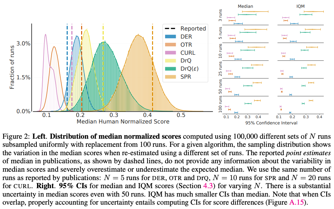
Remark. Following prior work, we recommend using confidence intervals for measuring the uncertainty in results and showing effect sizes (e.g. performance improvements over baseline) that are compatible with the given data. Furthermore, we emphasize using statistical thinking but avoid statistical significance tests (e.g. $p$-value < $0.05$) because of their dichotomous nature (significant versus not significant) and common misinterpretations such as 1) lack of statistically significant results does not demonstrate the absence of effect (see right panel of Figure 2, below), and 2) given enough data, any trivial effect can be statistically significant but may not be practically significant.
Case Study: The Atari 100k benchmark
We begin with a case study to illustrate the pitfalls arising from the naive use of point estimates in the few-run regime. Our case study concerns the Atari 100k benchmark, an offshoot of the ALE for evaluating data-efficiency in deep RL. In this benchmark, algorithms are evaluated on only 100k steps (2-3 hours of game-play) for each of its 26 games, versus 200M frames in the ALE benchmark. Prior reported results on this benchmark have been computed mostly from 3 or 5 runs, and more rarely, 10 or 20 runs.
Our case study compares the performance of five recent deep RL algorithms, namely: (1) DER, (2) OTR, (3) DrQ, (4) CURL, and (5) SPR. We chose these methods as representative of influential algorithms within this benchmark. Since good performance on one game can result in unduly high sample means without providing much information about performance on other games, it is common to measure performance on Atari 100k using sample medians. Refer to Appendix A.2 in the paper for more details about the experimental setup.
We investigate statistical variations in the few-run regime by evaluating 100 independent runs for each algorithm, where the score for a run is the average returns obtained in 100 evaluation episodes taking place after training. Each run corresponds to training one algorithm on each of the 26 games in Atari 100k. This provides us with $26 \times 100$ scores per algorithm, which we then subsample with replacement to 3–100 runs. The subsampled scores are then used to produce a collection of point estimates whose statistical variability can be measured. We begin by using this experimental protocol to highlight statistical concerns regarding median normalized scores.
High variability in reported results. Our first observation is that the sample medians reported in the literature exhibit substantial variability when viewed as random quantities that depend on a small number of sample runs (see left panel of figure below). This shows that there is a fairly large potential for drawing erroneous conclusions based on point estimates alone. As a concrete example, our analysis suggests that DER may in fact be better than OTR, unlike what the reported point estimates suggest. We conclude that in the few-run regime, point estimates are unlikely to provide definitive answers to the question: “Would we draw the same conclusions were we to re-evaluate our algorithm with a different set of runs?”
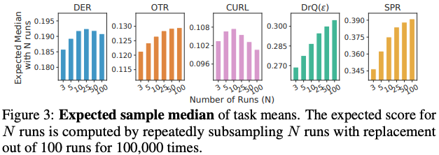
Substantial bias in sample medians. The sample median is a biased estimator of the true median: $\mathbb{E}[\text{Median}({\bar X}_{1:M})] \neq \text{Median}(\mathbb{E}[X_{1:M}])$ in general. In the few-run regime, we find that this bias can dominate the comparison between algorithms, as evidenced in the figure below. For example, the score difference between sample medians with 5 and 100 runs for SPR (+0.03 points) is about 36% of its mean improvement over DRQ $(\varepsilon)$ (+0.08 points). Adding to the issue, the magnitude and sign of this bias strongly depends on the algorithm being evaluated.
Statistical concerns cannot be satisfactorily addressed with few runs. While claiming improvements with 3 or fewer runs may naturally raise eyebrows, folk wisdom in experimental RL suggests that 20 or 30 runs are enough. By calculating 95% confidence interval (Specifically, we use the $m/n$ bootstrap to calculate the interval between $[2.5^{th}, 97.5^{th}]$ percentiles of the distribution of sample medians (95% CIs).) on sample medians for a varying number of runs (Figure 2 above, right), we find that this number is closer to 50–100 runs in Atari 100k – far too many to be computationally feasible for most research projects.
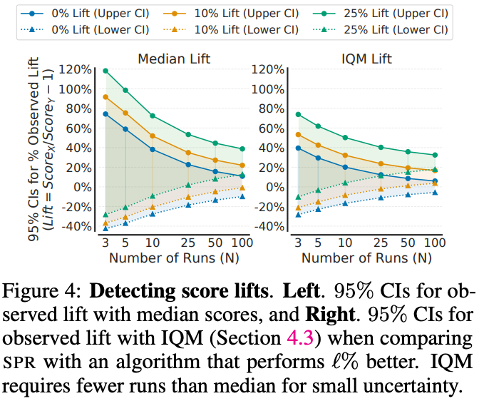
Consider a setting in which an algorithm is known to be better – what is the reliability of median and IQM for accurately assessing performance differences as the number of runs varies? Specifically, we consider two identical $N$-run experiments involving SPR, except that we artificially inflate one of the experiments’ scores by a fixed fraction or lift of $+\ell\%$ (see Figure 4 below). In particular, $\ell = 0$ corresponds to running the same experiment twice but with different runs. We find that statistically defensible improvements with median scores is only achieved for 25 runs~($\ell=25$) and 100 runs ($\ell=10$). With $\ell = 0$, even 100 runs are insufficient, with deviations of $20\%$ possible.
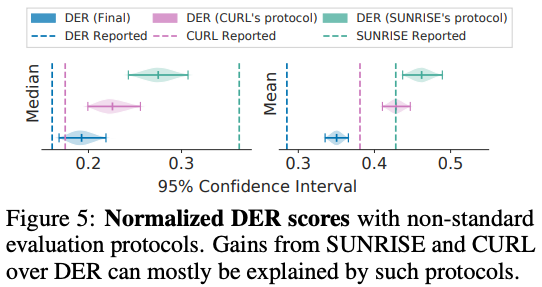
Changes in evaluation protocols invalidates comparisons to prior work. A typical and relatively safe approach for measuring the performance of an RL algorithm is to average the scores received in their final training episodes. However, the field has seen a number of alternative protocols used, including reporting the maximum evaluation score achieved during training or across multiple runs. A similar protocol is also used by CURL and SUNRISE (See Appendix A.4 in paper).
Results produced under alternative protocols involving maximum are generally incomparable with end-performance reported results. On Atari 100k, we find that the two protocols produce substantially different results (see Figure 5 below), of a magnitude greater than the actual difference in score. In particular, evaluating DER with CURL’s protocol results in scores far above those reported for CURL. In other words, this gap in evaluation procedures resulted in CURL being assessed as achieving a greater true median than DER, where our experiment gives strong support to DER being superior. Similarly, we find that a lot of SUNRISE’s improvement over DER can be explained by the change in evaluation protocol (see Figure 5 below). Refer to Appendix A.4 in the paper for discussion on pitfalls of such alternative protocols.
Recommendations and Tools for Reliable Evaluation
Our case study shows that the increase in the number of runs required to address the statistical uncertainty issues is typically infeasible for computationally demanding deep RL benchmarks. In this section, we identify three tools for improving the quality of experimental reporting in the few-run regime, all aligned with the principle of accounting for statistical uncertainty in results.
Stratified Bootstrap Confidence Intervals
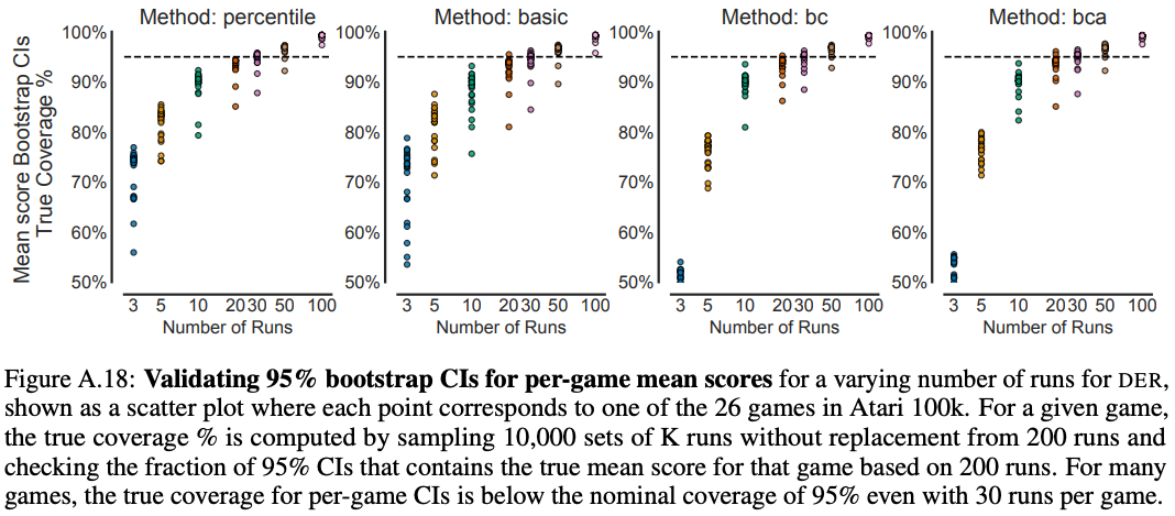
We first reaffirm the importance of reporting interval estimates to indicate the range within which an algorithm’s aggregate performance is believed to lie. Concretely, we propose using bootstrap CIs with stratified sampling for aggregate performance, a method that can be applied to small sample sizes and is better justified than reporting sample standard deviations in this context. While prior work has recommended using bootstrap CIs for reporting uncertainty in single task mean scores with $N$ runs, this is less useful when $N$ is small (see Figure A.18 below), as bootstrapping assumes that re-sampling from the data approximates sampling from the true distribution. We can do better by aggregating samples across tasks, for a total of $MN$ random samples.
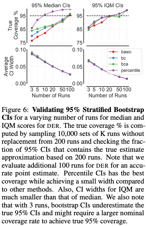
To compute the stratified bootstrap CIs, we re-sample runs with replacement independently for each task to construct an empirical bootstrap sample with $N$ runs each for $M$ tasks from which we calculate a statistic and repeat this process many times to approximate the sampling distribution of the statistic. We measure the reliability of this technique in Atari 100k for variable $N$, by comparing the nominal coverage of 95% to the “true” coverage from the estimated CIs (see Figure 6 below) for different bootstrap methods. We find that percentile CIs provide good interval estimates for as few as $N=10$ runs for both median and IQM scores.
Performance Profiles
Most deep RL benchmarks yield scores that vary widely between tasks and may be heavy-tailed, multimodal, or possess outliers (e.g. see Figure below). In this regime, both point estimates, such as mean and median scores, and interval estimates of these quantities paint an incomplete picture of an algorithm’s performance. Instead, we recommend the use of performance profiles, commonly used in benchmarking optimization software. While performance profiles from Dolan and Moré correspond to empirical cumulative distribution functions without any uncertainty estimates, profiles proposed herein visualize the empirical tail distribution function of a random score (higher curve is better), with pointwise confidence bands based on stratified bootstrap.
By representing the entire set of normalized scores $x_{1:M, 1:N}$ visually, performance profiles reveal performance variability across tasks much better than interval estimates of aggregate metrics. Although tables containing per-task mean scores and standard deviations can reveal this variability, such tables tend to be overwhelming for more than a few tasks. In addition, performance profiles are robust to outlier runs and insensitive to small changes in performance across all tasks.
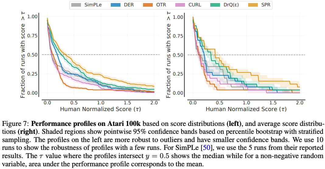
In this paper, we propose the use of a performance profile we call run-score distributions or simply score distributions (Figure 7 below, right), particularly well-suited to the few-run regime. A score distribution shows the fraction of runs above a certain normalized score and is given by
$$ \hat{F}_X(\tau) = \hat{F}(\tau; x_{1:M, 1:N}) = \frac{1}{M} \sum_{m=1}^{M} \hat{F}_m(\tau) = \frac{1}{M} \sum_{m=1}^{M} \frac{1}{N} \sum_{n=1}^{N} \mathbb{1}[x_{m,n} > \tau] $$
One advantage of the score distribution is that it is an unbiased estimator of the underlying distribution $F(\tau) = \tfrac{1}{N} \sum_{m=1}^{M} F_{m}(\tau)$. Another advantage is that an outlier run with extremely high score can change the output of score distribution for any $\tau$ by at most a value of $\tfrac{1}{MN}$.
It is useful to contrast score distributions to average-score distributions, originally proposed in the context of the ALE as a generalization of the median score. Average-score distributions correspond to the performance profile of a random variable $\bar{X}$, $\hat{F}_{\bar{X}}(\tau) = \hat{F}(\tau; {\bar x}_{1:M})$, which shows the fraction of tasks on which an algorithm performs better than a certain score. However, such distributions are a biased estimate of the thing they seek to represent. Run-score distributions are more robust than average-score distributions, as they are a step function in $1/MN$ versus $1/M$ intervals, and typically has less variance: $\sigma_X^2 = \tfrac{1}{M^2N} \sum_{m=1}^{M} F_m(\tau)(1 - F_m(\tau))$ versus $\sigma_{\bar X}^2 = \tfrac{1}{M^2}\sum_{m=1}^{M} F_{\bar{X}_{m}}(\tau)(1 - F_{\bar{X}_m}(\tau))$. Figure 7 below illustrates these differences.
Robust and Efficient Aggregate Metrics
Performance profiles allow us to compare different methods at a glance. If one curve is strictly above another, the better method is said to stochastically dominate the other. In RL benchmarks with a large number of tasks, however, stochastic dominance is rarely observed: performance profiles often intersect at multiple points. Finer quantitative comparisons must therefore entail aggregate metrics.
We can extract a number of aggregate metrics from score distributions, including median (mixing runs and tasks) and mean normalized scores (matching our usual definition). As we already argued that these metrics are deficient, we now consider interesting alternatives also derived from score distributions.
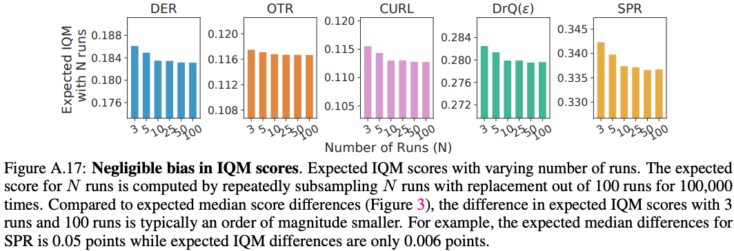
As an alternative to median, we recommend using the interquartile mean (IQM). Also called 25% trimmed mean, IQM discards the bottom and top $25\%$ of the runs and calculates the mean score of the remaining 50% runs (=$\lfloor NM/2 \rfloor$ for $N$ runs each on $M$ tasks). IQM interpolates between mean and median across runs, which are 0% and almost $50%$ trimmed means respectively. Compared to sample median, IQM is a better indicator of overall performance as it is calculated using 50% of the combined runs while median only depends on the performance ordering across tasks and not on the magnitude except at most 2 tasks. For example, zero scores on nearly half of the tasks does not affect the median while IQM exhibits a severe degradation. Compared to mean, IQM is robust to outliers, yet has considerably less bias than median (see Figure A.17 below). While median is more robust to outliers than IQM, this robustness comes at the expense of statistical efficiency, which is crucial in the few-run regime: IQM results in much smaller CIs (Figure 2 (right) and Figure 6) and is able to detect a given improvement with far fewer runs (Figure 4).
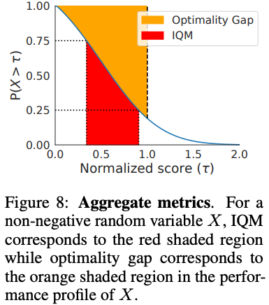
As a robust alternative to mean, we recommend using the optimality gap: the amount by which the algorithm fails to meet a minimum score of $\gamma = 1.0$ (orange region in Figure 8 below). This assumes that a score of 1.0 is a desirable target beyond which improvements are not very important, for example when the aim is to obtain human-level performance. Naturally, the threshold $\gamma$ may be chosen differently, which we discuss further in Appendix A.7 in the paper.
If one is interested in knowing how robust an improvement from an algorithm $X$ over an algorithm $Y$ is, another possible metric to consider is the average probability of improvement – this metric shows how likely it is for $X$ to outperform $Y$ on a randomly selected task. Specifically, $P(X > Y) = \tfrac{1}{M} \sum_{m=1}^{M} P(X_m > Y_m)$, where $P(X_m > Y_m)$ (Equation A.2 in paper) is the probability that $X$ is better than $Y$ on task $m$. Note that, unlike IQM and optimality gap, this metric does not account for the size of improvement. While finding the best aggregate metric is still an open question and is often dependent on underlying normalized score distribution, our proposed alternatives avoid the failure modes of prevalent metrics while being robust and requiring fewer runs to reduce uncertainty.
Re-evaluating Evaluation on Deep RL Benchmarks
Arcade Learning Environment
Training RL agents for 200M frames on the ALE is the most widely recognized benchmark in deep RL. We revisit some popular methods which demonstrated progress on this benchmark and reveal discrepancies in their findings as a consequence of ignoring the uncertainty in their results (Figure 9 below). For example, DreamerV2 exhibits a large amount of uncertainty in aggregate scores. While M-IQN claimed better performance than Dopamine Rainbow (Dopamine Rainbow differs from the original by not including double DQN, dueling architecture and noisy networks. Also, results in the original Rainbow paper were reported using a single run without sticky actions.) in terms of median normalized scores, their interval estimates strikingly overlap. Similarly, while C51 is considered substantially better than DQN, the interval estimates as well as performance profiles for DQN (Adam) and C51 overlap significantly.
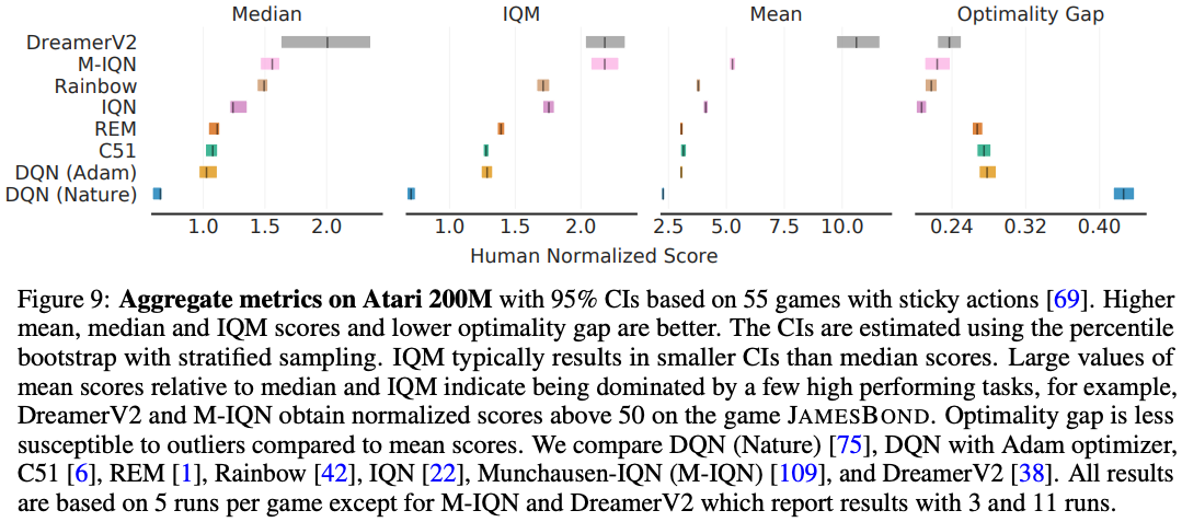
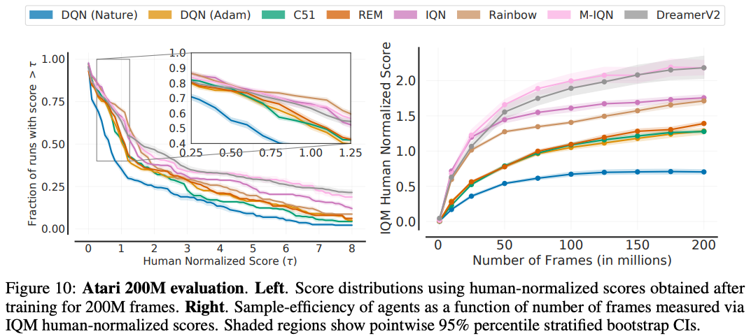
Figure 9 below reveals an interesting limitation of aggregate metrics: depending on the choice of metric, the ordering between algorithms changes (e.g. Median vs. IQM). The inconsistency in ranking across aggregate metrics arises from the fact that such metrics only capture a specific aspect of overall performance across tasks and runs. Additionally, the change of algorithm ranking between optimality gap and IQM/median scores reveal that while recent algorithms typically show performance gains relative to humans on average, their performance seems to be worse on games below human performance. Since performance profiles capture the full picture, they would often illustrate why such inconsistencies exist. For example, optimality gap and IQM can be both read as areas in the profile (Figure 8). The performance profile in Figure 10 (left) illustrates the nuances present when comparing different algorithms. For example, IQN seems to be better than Rainbow for $\tau \geq 2$, but worse for $\tau < 2$. Similarly, the profiles of DreamerV2 and M-IQN for $\tau < 8$ intersect at multiple points. To compare sample efficiency of the agents, we also present their IQM scores as a function of number of frames in Figure 10 (right).
DeepMind Control Suite
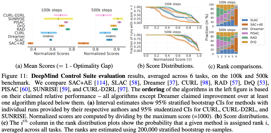
Recent continuous control papers benchmark performance on 6 tasks in DM Control at 100k and 500k steps. Typically, such papers claim improvement based on higher mean scores per task regardless of the variability in those scores. However, we find that when accounting for uncertainty in results, most algorithms do not consistently rank above algorithms they claimed to improve upon (Figure 11c and 11b). Furthermore, there are huge overlaps in 95% CIs of mean normalized scores for most algorithms (Figure 11a). These findings suggest that a lot of the reported improvements are spurious, resulting from randomness in the experimental protocol.
Procgen benchmark
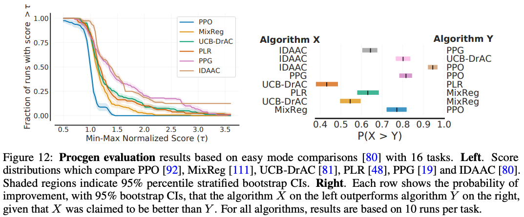
Procgen is a popular benchmark, consisting of 16 diverse tasks, for evaluating generalization in RL. Recent papers report mean PPO-normalized scores on this benchmark to emphasize the gains relative to PPO as most methods are built on top of it. However, Figure 12 (left) shows that PPO-normalized scores typically have a heavy-tailed distribution making the mean scores highly dependent on performance on a small fraction of tasks.
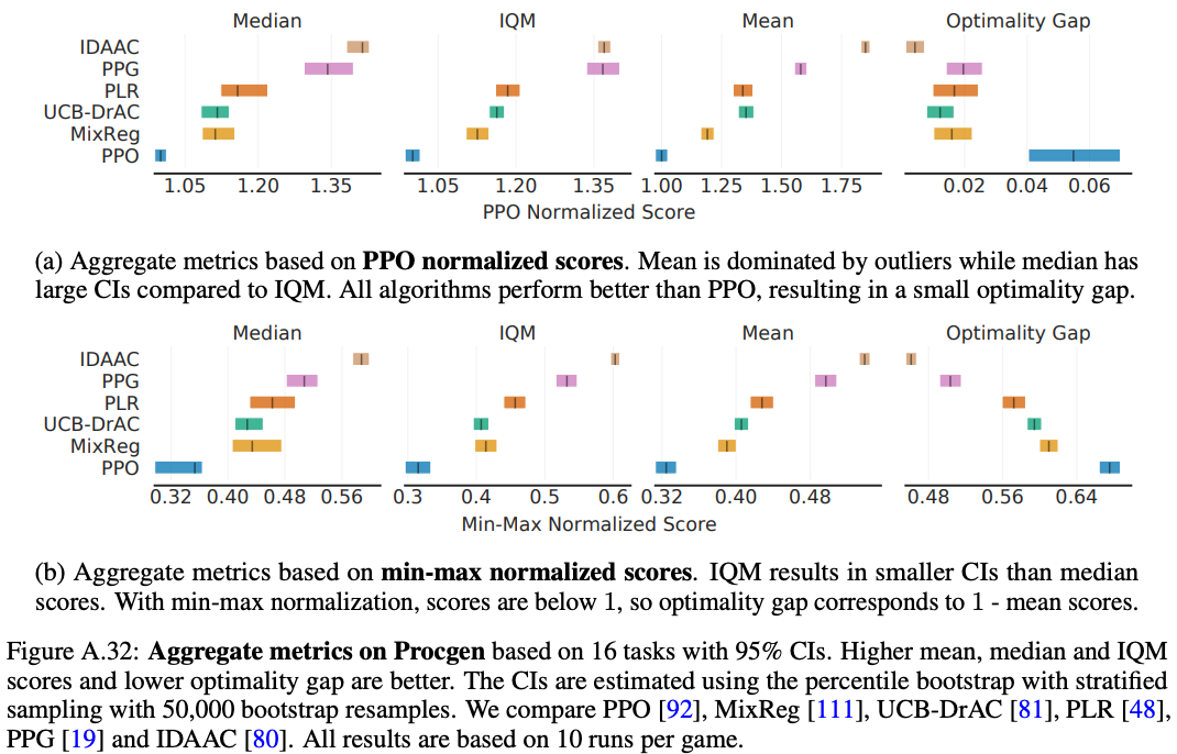
Instead, we recommend using normalization based on the estimated minimum and maximum scores on ProcGen and reporting aggregate metrics based on such scores (Figure A.32 below).
While publications sometimes make binary claims about whether they improve over prior methods, such improvements are inherently probabilistic. To reveal this discrepancy, we investigate the following question: “What is the probability that an algorithm which claimed improvement over a prior algorithm performs better than it?” (Figure 12, right). While this probability does not distinguish between two algorithms which uniformly improve on all tasks by 1% and 100%, it does highlight how likely an improvement is. For example, there is only a $40-50$% chance that UCB-DrAC improves upon PLR. We note that a number of improvements reported in the existing literature are only $50-70$% likely.
Discussion
We saw, both in our case study on the Atari 100k benchmark and with our analysis of other widely-used RL benchmarks, that statistical issues can have a sizeable influence on reported results, in particular when point estimates are used or evaluation protocols are not kept constant within comparisons. Despite earlier calls for more experimental rigor in deep RL, our analysis shows that the field has not yet found sure footing in this regards.
In part, this is because the issue of reproducibility is a complex one; where our work is concerned with our confidence about and interpretation of reported results (what Goodman et al. calls results reproducibility), others have highlighted that there might be missing information about the experiments themselves (methods reproducibility). We remark that the problem is not solved by fixing random seeds, as has sometimes been proposed, since it does not really address the question of whether an algorithm would perform well under similar conditions but with different seeds. Furthermore, fixed seeds might benefit certain algorithms more than others. Nor can the problem be solved by the use of dichotomous statistical significance tests, as discussed above.
One way to minimize the risks associated with statistical effects is to report results in a more complete fashion, paying close attention to bias and uncertainty within these estimates. To this end, our recommendations are summarized in Table 1 above. To further support RL researchers in this endeavour, we released an easy-to-use Python library, RLiable along with a Colab notebook for implementing our recommendations, as well as all the individual runs used in our experiments. Again, we emphasize the importance of published papers providing results for all runs to allow for future statistical analyses.
A barrier to adoption of evaluation protocols proposed in this work, and more generally, rigorous evaluation, is whether there are clear incentives for researchers to do so, as more rigor generally entails more nuanced and tempered claims. Arguably, doing good and reproducible science is one such incentive. We hope that our findings about erroneous conclusions in published papers would encourage researchers to avoid fooling themselves, even if that requires tempered claims. That said, a more pragmatic incentive would be if conferences and reviewers required more rigorous evaluation for publication, e.g. NeurIPS 2021 checklist asks whether error bars are reported. Moving towards reliable evaluation is an ongoing process and we believe that this paper would greatly benefit it.
Given the substantial influence of statistical considerations in experiments involving 40-year old Atari 2600 video games and low-DOF robotic simulations, we argue that it is unlikely that an increase in available computation will resolve the problem for the future generation of RL benchmarks. Instead, just as a well-prepared rock-climber can skirt the edge of the steepest precipices, it seems likely that ongoing progress in reinforcement learning will require greater experimental discipline.
comments powered by Disqus