
Pablo Samuel Castro
October 21, 2021
MICo: Learning improved representations via sampling-based state similarity for Markov decision processes
We present a new behavioural distance over the state space of a Markov decision process, and demonstrate the use of this distance as an effective means of shaping the learnt representations of deep reinforcement learning agents.
Pablo Samuel Castro*, Tyler Kastner*, Prakash Panangaden, and Mark Rowland
This blogpost is a summary of our NeurIPS 2021 paper. The code is available here.
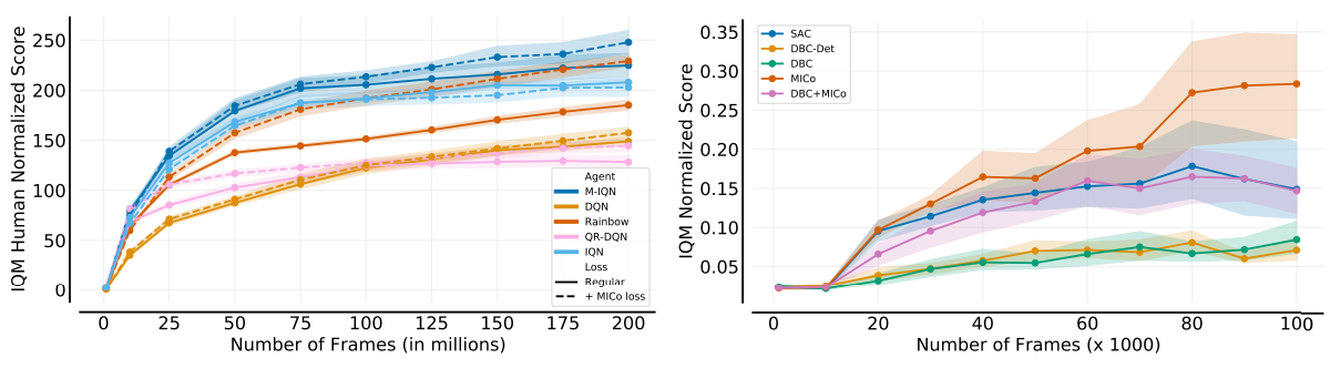
The following figure gives a nice summary of the empirical gains our new loss provides, yielding an improvement on all of the Dopamine agents (left), as well as over Soft Actor-Critic and the DBC algorithm of Zhang et al., ICLR 2021 (right). In both cases we are reporting the Interquantile Mean as introduced in our Statistical Precipice NeurIPS'21 paper.
Introduction
The success of reinforcement learning (RL) algorithms in large-scale, complex tasks depends on forming useful representations of the environment with which the algorithms interact. Feature selection and feature learning has long been an important subdomain of RL, and with the advent of deep reinforcement learning there has been much recent interest in understanding and improving the representations learnt by RL agents.
We introduce the MICo (Matching under Independent Couplings) distance, and develop the theory around its computation and estimation, making comparisons with existing metrics on the basis of computational and statistical efficiency. We empirically demonstrate that directly shaping the representation with MICo (as opposed to implicitly as most previous methods) yields improvements on a number of value-based deep RL agents.
Expand to read more details
Much of the work in representation learning has taken place from the perspective of auxiliary tasks [Jaderberg et al., 2017], [Fedus et al., 2019]; in addition to the primary reinforcement learning task, the agent may attempt to predict and control additional aspects of the environment. Auxiliary tasks shape the agent’s representation of the environment implicitly, typically via gradient descent on the additional learning objectives. As such, while auxiliary tasks continue to play an important role in improving the performance of deep RL algorithms, our understanding of the effects of auxiliary tasks on representations in RL is still in its infancy.
In contrast to the implicit representation shaping of auxiliary tasks, a separate line of work on behavioural metrics, such as bisimulation metrics [Desharnais et al., 1999], [Ferns et al., 2004], aims to capture structure in the environment by learning a metric measuring behavioral similarity between states. Recent works have successfully used behavioural metrics to shape the representations of deep RL agents [Gelada et al., 2019], [Zhang et al., 2021], [Agarwal et al., 2021]. However, in practice behavioural metrics are difficult to estimate from both statistical and computational perspectives, and these works either rely on specific assumptions about transition dynamics to make the estimation tractable, and as such can only be applied to limited classes of environments, or are applied to more general classes of environments not covered by theoretical guarantees.
The principal objective of this work is to develop new measures of behavioral similarity that avoid the statistical and computational difficulties described above, and simultaneously capture richer information about the environment.
Background
To streamline the reading of this post, I’ve made the details in the background section collapsible. Click on each section header to read more.
Reinforcement learning
Reinforcement learning methods are used for sequential decision making in uncertain environments. You can read an introduction to reinforcement learning in this post, or expand the section below for more details.
More details
Denoting by $\mathscr{P}(S)$ the set of probability distributions on a set $S$, we define a Markov decision process $(\mathcal{X}, \mathcal{A}, \gamma, P, r)$ as:
- A finite state space $\mathcal{X}$;
- A finite action space $\mathcal{A}$;
- A transition kernel $P : \mathcal{X} \times \mathcal{A}\rightarrow \mathscr{P}(\mathcal{X})$;
- A reward function $r : \mathcal{X} \times\mathcal{A} \rightarrow \mathbb{R}$;
- A discount factor $\gamma \in [0,1)$.
For notational convenience we introduce the notation $P_x^a \in \mathscr{P}(\mathcal{X})$ for the next-state distribution given state-action pair $(x, a)$, and $r_x^a$ for the corresponding immediate reward.
Policies are mappings from states to distributions over actions: $\pi \in \mathscr{P}(\mathcal{A})^\mathcal{X}$ and induce a value function $V^{\pi}:\mathcal{X}\rightarrow\mathbb{R}$ defined via the recurrence:
$$V^{\pi}(x) := \mathbb{E}_{a\sim\pi(x)}\left[ r_x^a + \gamma\mathbb{E}_{x’\sim P_x^a} [V^{\pi}(x’)]\right]$$
It can be shown that this recurrence uniquely defines $V^\pi$ through a contraction mapping argument.
The control problem is concerned with finding the optimal policy
$$ \pi^{*} = \arg\max_{\pi\in\mathscr{P}(\mathcal{A})^\mathcal{X}}V^{\pi} $$
It can be shown that while the optimisation problem above appears to have multiple objectives (one for each coordinate of $V^\pi$, there is in fact a policy $\pi^{*} \in \mathscr{P}(\mathcal{A})^\mathcal{X}$ that simultaneously maximises all coordinates of $V^\pi$, and that this policy can be taken to be deterministic; that is, for each $x \in \mathcal{X}$, $\pi(\cdot|x) \in \mathscr{P}(\mathcal{A})$ attributes probability 1 to a single action. In reinforcement learning in particular, we are often interested in finding, or approximating, $\pi^{*}$ from direct interaction with the MDP in question via sample trajectories, without knowledge of $P$ or $r$ (and sometimes not even $\mathcal{X}$).
Bisimulation metrics
Bisimulation metrics quantify the behavioural distance between two states in a Markov decision process. I give a brief introduction to bisimulation metrics in this post, or you can read more details by expanding the section below.
More details
A metric $d$ on a set $X$ is a function $d:X\times X\rightarrow [0, \infty)$ respecting the following axioms for any $x, y, z \in X$:
- Identity of indiscernibles: $d(x, y) = 0 \iff x = y$;
- Symmetry: $d(x, y) = d(y, x)$;
- Triangle inequality: $d(x, y) \leq d(x, z) + d(z, y)$.
A pseudometric is similar, but the “identity of indiscernibles” axiom is weakened:
- $x = y \implies d(x, y) = 0$;
- $d(x, y) = d(y, x)$;
- $d(x, y) \leq d(x, z) + d(z, y)$.
Note that the weakened first condition does allow one to have $d(x, y) = 0$ when $x\ne y$.
A (pseudo)metric space $(X, d)$ is defined as a set $X$ together with a (pseudo)metric $d$ defined on $X$.
Bisimulation is a fundamental notion of behavioural equivalence introduced by Park and Milner in the early 1980s in the context of nondeterministic transition systems. The probabilistic analogue was introduced by Larsen and Skou. The notion of an equivalence relation is not suitable to capture the extent to which quantitative systems may resemble each other in behaviour. To provide a quantitative notion, bisimulation metrics were introduced by [Desharnais et al., 1999] in the context of probabilistic transition systems without rewards. In reinforcement learning the reward is an important ingredient, accordingly the bisimulation metric for states of MDPs was introduced by [Ferns et al., 2004].
Various notions of similarity between states in MDPs have been considered in the RL literature, with applications in policy transfer, state aggregation, and representation learning. The bisimulation metric is of particular relevance for this paper, and defines state similarity in an MDP by declaring two states $x,y \in \mathcal{X}$ to be close if their immediate rewards are similar, and the transition dynamics at each state leads to next states which are also judged to be similar.
Central to the definition of the bisimulation metric is the operator $T_k : \mathcal{M}(\mathcal{X}) \rightarrow \mathcal{M}(\mathcal{X})$, defined over $\mathcal{M}(\mathcal{X})$, the space of pseudometrics on $\mathcal{X}$. We now turn to the definition of the operator itself, given by
$$T_k(d)(x, y) = \max_{a \in \mathcal{A}} [|r_x^a - r_y^a] + \gamma W_d(P^a_x, P^a_y)]$$
for each $d \in \mathcal{M}(\mathcal{X})$, and each $x, y \in \mathcal{X}$. It can be verified that the function $T_K(d) : \mathcal{X} \times \mathcal{X} \rightarrow \mathbb{R}$ satisfies the properties of a pseudometric, so under this definition $T_K$ does indeed map $\mathcal{M}(\mathcal{X})$ into itself.
The other central mathematical concept underpinning the operator $T_K$ is the Kantorovich distance $W_d$ (Commonly known as the Wasserstein distance) using base metric $d$. $W_d$ is formally a pseudometric over the set of probability distributions $\mathscr{P}(\mathcal{X})$, defined as the solution to an optimisation problem. The problem specifically is formulated as finding an optimal coupling between the two input probability distributions that minimises a notion of transport cost associated with $d$. Mathematically, for two probability distributions $\mu, \mu’ \in \mathscr{P}(\mathcal{X})$, we have \begin{align*} W_d(\mu, \mu’) = \min_{\substack{(Z, Z’) \ Z \sim \mu, Z’ \sim \nu’}} \mathbb{E}[d(Z, Z’)] , . \end{align*} Note that the pair of random variables $(Z, Z’)$ attaining the minimum in the above expression will in general not be independent. That the minimum is actually attained in the above example in the case of a finite set $\mathcal{X}$ can be seen by expressing the optimisation problem as a linear program. Minima are obtained in much more general settings too; see Cedric Villani’s book for more details.
The operator $T_K$ can be analysed in a similar way to standard operators in dynamic programming for reinforcement learning. It can be shown that it is a contraction mapping with respect to the $L^\infty$ metric over $\mathcal{M}(\mathcal{X})$, and that $\mathcal{M}(\mathcal{X})$ is a complete metric space with respect to the same metric. Thus, by Banach’s fixed point theorem, $T_K$ has a unique fixed point in $\mathcal{M}(\mathcal{X})$, and repeated application of $T_K$ to any initial pseudometric will converge to this fixed point.
Finally, Ferns et al. show that this metric bounds differences in the optimal value function, hence its importance in RL:
$$|V^{*}(x) - V^{*}(y)| \leq d^\sim(x, y) \quad \forall x,y\in\mathcal{X}$$
Representation learning in RL
In large-scale environments, RL agents must approximate value functions in a more concise manner, by forming a representation of the environment.
More details
In large-scale environments, it is infeasible to express value functions directly as vectors in $\mathbb{R}^{\mathcal{X} \times \mathcal{A}}$. Instead, RL agents must approximate value functions in a more concise manner, by forming a representation of the environment, that is, a feature embedding $\phi: \mathcal{X} \rightarrow \mathbb{R}^M$, and predicting state-action values linearly from these features. Representation learning is the problem of finding a useful representation $\phi$. Increasingly, deep RL agents are equipped with additional losses to aid representation learning. A common approach is to require the agent to make additional predictions (so-called auxilliary tasks) with its representation, typically with the aid of extra network parameters, with the intuition that an agent is more likely to learn useful features if it is required to solve many related tasks. We refer to such methods as implicit representation shaping, since improved representations are a side-effect of learning to solve auxiliary tasks.
Since bisimulation metrics capture additional information about the MDP in addition to that summarised in value functions, bisimulation metrics are a natural candidate for auxiliary tasks in deep reinforcement learning. Gelada et al. [2019], Zhang et al. [2021], and Agarwal et al. [2021] introduce auxiliary tasks based on bisimulation metrics, but require additional assumptions on the underlying MDP in order for the metric to be learnt correctly (Lipschitz continuity, deterministic, and Gaussian transitions, respectively). The success of these approaches provides motivation in this paper to introduce a notion of state similarity applicable to arbitrary MDPs, without further restriction. Further, we learn this state similarity explicitly: that is, without the aid of any additional network parameters.
Limitations of bisimulation metrics
Bisimulation metrics provide a strong notion of distance on the state space of an MDP; however, they have been difficult to use at scale and compute online, including the following reasons:
Computational complexity
The metric can be computed via fixed-point iteration since the operator $T_K$ is a contraction mapping. The map $T_K$ contracts at rate $\gamma$ with respect to the $L^\infty$ norm on $\mathcal{M}$, and therefore obtaining an $\varepsilon$-approximation of $d^\sim$ under this norm requires $O(\log(\varepsilon) / \log(\gamma))$ applications of $T_K$ to an initial pseudometric $d_0$. The cost of each application of $T_K$ is dominated by the computation of $|\mathcal{X}|^2|\mathcal{A}|$ $W_d$ distances for distributions over $\mathcal{X}$, each costing $\tilde{O}(|\mathcal{X}|^{2.5})$ in theory, and $\tilde{O}(|\mathcal{X}|^3)$ in practice. Thus, the overall practical cost is $\tilde{O}(|\mathcal{X}|^{5}|\mathcal{A}|\log(\varepsilon) / \log(\gamma))$.
This property expresses the intrinsic computational difficulty of computing this metric.
Bias under sampled transitions.
Computing $T_K$ requires access to the transition probability distributions $P_x^a$ for each $(x, a) \in \mathcal{X} \times \mathcal{A}$ which, as mentioned above, are typically not available; instead, stochastic approximations to the operator of interest are employed. Whilst there has been work in studying online, sample-based approximate computation of the bisimulation metric, these methods are generally biased, in contrast to sample-based estimation of standard RL operators.
This property illustrates the problems associated with attempting to move from operator-based computation to online, sampled-based computation of the metric (for example, when the environment dynamics are unknown).
Lack of connection to non-optimal policies
One of the principal behavioural characterisations of the bisimulation metric $d^\sim$ is the upper bound shown above. However, in general we do not have
$$|V^\pi(x) - V^\pi (y)| \leq d^\sim(x, y)$$
for arbitrary policies $\pi \in \Pi$; a simple example is illustrated below:
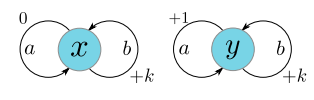
In this MDP, $d^\sim(x, y) = (1-\gamma)^{-1}$, but for the policy $\pi(b|x)=1, \pi(a|y) = 1$, we have $|V^\pi(x) - V^\pi(y)| = k(1-\gamma)^{-1}$.
More generally, notions of state similarity that the bisimulation metric encodes may not be closely related to behavioural similarity under the policy $\pi$. Thus, learning about $d^\sim$ may not in itself be useful for large-scale reinforcement learning agents.
This property shows that even if the metric is computable exactly, the information it yields about the MDP may not be practically useful. Although $\pi$-bisimulation (introduced by me here) and extended by Zhang et al. [2021]) addresses this property, their practical algorithms are limited to MDPs with deterministic transitions or MDPs with Gaussian transition kernels, respectively.
The MICo distance
We now present a new notion of distance for state similarity, which we refer to as MICo (M_atching under _I_ndependent _Couplings), designed to overcome the drawbacks described above. We make some modifications to $T_K$ to deal with the previously mentioned shortcomings, detailed below.
In order to deal with the prohibitive cost of computing the Kantorovich distance, which optimizes over all coupling of the distributions $P_x^a$ and $P_y^a$, we use the independent coupling.
To deal with lack of connection to non-optimal policies, we consider an on-policy variant of the metric, pertaining to a chosen policy $\pi \in \mathscr{P}(\mathcal{A})^\mathcal{X}$. This leads us to the following definition.
Definition
Given a policy $\pi \in\mathscr{P}(\mathcal{A})^\mathcal{X}$, the MICo update operator, $T^\pi_M : \mathbb{R}^{\mathcal{X}\times\mathcal{X}} \rightarrow \mathbb{R}^{\mathcal{X}\times\mathcal{X}}$, is defined by
$$(T^\pi_M U)(x, y) = |r^\pi_x - r^\pi_y| + \gamma \mathbb{E}_{\begin{subarray}{l}x’\sim P^{\pi}_x \ y’\sim P^{\pi}_y\end{subarray}} \left[ U(x’, y’) \right]$$
for all functions $U:\mathcal{X}\times\mathcal{X}\rightarrow\mathbb{R}$, with $r^\pi_x = \sum_{a \in \mathcal{A}} \pi(a|x) r_x^a$ and $P^{\pi}_x = \sum_{a\in\mathcal{A}}\pi(a|x)P_x^a(\cdot)$ for all $x \in \mathcal{X}$.
As with the bisimulation operator, this can be thought of as encoding desired properties of a notion of similarity between states in a self-referential manner; the similarity of two states $x, y \in \mathcal{X}$ should be determined by the similarity of the rewards and the similarity of the states they lead to.
Proposition
The MICo operator $T^\pi_M$ is a contraction mapping on $\mathbb{R}^{\mathcal{X}\times\mathcal{X}}$ with respect to the $L^\infty$ norm.
Proof
Let $U, U’ \in \mathbb{R}^{\mathcal{X}\times\mathcal{X}}$. Then note that
$$|(T^\pi U)(x, y) - (T^\pi U’)(x, y)| = \left|\gamma\sum_{x’, y’}\pi(a|x)\pi(b|y)P_x^a(x’)P_y^b(y’) (U - U’)(x’, y’) \right| \leq \gamma |U - U’|_\infty$$
for any $x,y \in \mathcal{X}$, as required.
The following corollary now follows immediately from Banach’s fixed-point theorem and the completeness of $\mathbb{R}^{\mathcal{X}\times\mathcal{X}}$ under the $L^\infty$ norm.
Corollary
The MICo operator $T^\pi_M$ has a unique fixed point $U^\pi \in \mathbb{R}^{\mathcal{X}\times\mathcal{X}}$, and repeated application of $T^\pi_M$ to any initial function $U \in \mathbb{R}^{\mathcal{X}\times\mathcal{X}}$ converges to $U^\pi$.
Having defined a new operator, and shown that it has a corresponding fixed-point, there are two questions to address:
- Does this new notion of distance overcome the drawbacks of the bisimulation metric described above?
- What does this new object tell us about the underlying MDP?
Addressing the drawbacks of the bisimulation metric
In this section, we provide a series of results that show that the newly-defined notion of distance addressess each of these shortcomings presented previously. The proofs of these results rely on the following lemma, connecting the MICo operator to a lifted MDP.
Lemma (Lifted MDP)
The MICo operator $T^\pi_M$ is the Bellman evaluation operator for an auxiliary MDP.
Proof
Given the MDP specified by the tuple $(\mathcal{X}, \mathcal{A}, P, R)$, we construct an auxiliary MDP $(\widetilde{\mathcal{X}},\widetilde{\mathcal{A}}, \widetilde{P}, \widetilde{R})$ defined by: * State space $\widetilde{\mathcal{X}} = \mathcal{X}^2$ * Action space $\widetilde{\mathcal{A}} = \mathcal{A}^2$ * Transition dynamics given by $\widetilde{P}\_{(u, v)}^{(a, b)}((x,y)) = P\_u^a(x)P\_v^b(y)$ for all $(x,y), (u,v) \in \mathcal{X}^2$, $a,b \in \mathcal{A}$ * Action-independent rewards $\widetilde{R}\_{(x,y)} = |r^\pi\_x - r^\pi\_y|$ for all $x, y \in \mathcal{X}$.The Bellman evaluation operator $\widetilde{T}^{\tilde{\pi}}$ for this auxiliary MDP at discount rate $\gamma$ under the policy $\tilde{\pi}(a,b|x,y) = \pi(a|x) \pi(b|y)$ is given by: $$ (\widetilde{T}^{\tilde{\pi}}U)(x,y) = \widetilde{R}_{(x,y)} + \gamma \sum_{(x^\prime, y^\prime) \in \mathcal{X}^2} \widetilde{P}_{(x, y)}^{(a, b)}((x^\prime, y^\prime)) \tilde{\pi}(a,b|x,y) U(x^\prime, y^\prime)$$ $$ \qquad = |r^\pi_x - r^\pi_y| + \gamma \sum_{(x^\prime, y^\prime) \in \mathcal{X}^2} P^\pi_x(x^\prime)P_y^\pi(y^\prime) U(x^\prime, y^\prime)$$ $$ = (T^\pi_MU)(x, y) \qquad\qquad \qquad\qquad \qquad\quad$$
for all $U \in \mathbb{R}^{\mathcal{X}\times\mathcal{X}}$ and $(x, y) \in \mathcal{X} \times\mathcal{X}$, as required.
Equipped with the above lemma, we can address the three limitations listed above:
Computational complexity
Proposition
The computational complexity of computing an $\varepsilon$-approximation in $L^\infty$ to the MICo metric is $O(|\mathcal{X}|^4 \log(\varepsilon) / \log(\gamma))$.
Proof
Since the operator $T^\pi_M$ is a $\gamma$-contraction under $L^\infty$, we require $\mathcal{O}(\log(\varepsilon) / \log(\gamma))$ applications of the operator to obtain an $\varepsilon$-approximation in $L^\infty$. Each iteration of value iteration updates $|\mathcal{X}|^2$ table entries, and the cost of each update is $\mathcal{O}(|\mathcal{X}|^2)$, leading to an overall cost of $O(|\mathcal{X}|^4\log(\varepsilon) / \log(\gamma))$.
In contrast to the bisimulation metric, this represents a computational saving of $O(|\mathcal{X}|)$, which arises from the lack of a need to solve optimal transport problems over the state space in computing the MICo distance. There is a further saving of $\mathcal{O}(|\mathcal{A}|)$ that arises since MICo focuses on an individual policy $\pi$, and so does not require the max over actions in the bisimulation operator definition.
Online approximation
Proposition
Suppose rewards depend only on state, and consider the sequence of estimates $(U_t)_{t \geq 0}$, with $U_0$ initialised arbitrarily, and $U_{t+1}$ updated from $U_t$ via a pair of transitions $(x_t, a_t, r_t, x’_t)$, $(y_t, b_t, \tilde{r}_t, y’_t)$ as: $$U_{t+1}(x, y) \leftarrow (1-\epsilon_t(x, y))U_t(x, y) + \epsilon_t(x, y) ( |r - \tilde{r}| + \gamma U_{t}(x’, y’) )$$ Suppose all state-pairs tuples are updated infinitely often, and stepsizes for these updates satisfy the Robbins-Monro conditions. Then $U_t \rightarrow U^\pi$ almost surely.
Proof
Due to the interpretation of the MICo operator $T^\pi_M$ as the Bellman evaluation operator in an auxiliary MDP, algorithms and associated proofs of correctness for computing the MICo distance online can be straightforwardly derived from standard online algorithms for policy evaluation. Under the assumptions of the proposition, the update described is exactly a TD(0) update in the lifted MDP described above. We can therefore appeal to Proposition~4.5 of Bertsekas and Tsitsiklis [1996] to obtain the result. Note that the wide range of online policy evaluation methods incorporating off-policy corrections and multi-step returns, as well as techniques for applying such methods at scale, may also be used.
Relationship to underlying policy
Proposition
For any policy $\pi \in \mathscr{P}(\mathcal{A})^{\mathcal{X}}$ and states $x,y \in \mathcal{X}$, we have $|V^\pi(x) - V^\pi(y)| \leq U^\pi(x, y)$.
Proof
We apply a coinductive argument [Kozen, 2007] to show that if \begin{align}\label{eq:pf1} |V^\pi(x) - V^\pi(y)| \leq U(x, y) \ \text{for all } x, y \in \mathcal{X} , \end{align} for some $U \in \mathbb{R}^{\mathcal{X}\times\mathcal{X}}$ symmetric in its two arguments, then we also have $$|V^\pi(x) - V^\pi(y)| \leq (T^\pi_M U)(x, y) \ \text{for all } x, y \in \mathcal{X}$$
Since the hypothesis holds for the constant function $U(x,y) = 2 R_\text{max}/(1-\gamma)$, and $T^\pi_M$ contracts around $U^\pi$, the conclusion then follows. Therefore, suppose the coinductive hypothesis holds. Then we have $$V^\pi(x) - V^\pi(y) = r^\pi_xx - r^\pi_y + \gamma \sum_{x’ \in \mathcal{X}} P^\pi_x(x’) V(x’) - \gamma \sum_{y’ \in \mathcal{X}} P^\pi_y(y’) V(y’) $$ $$\leq |r^\pi_x - r^\pi_y| + \gamma \sum_{x’, y’ \in \mathcal{X}} P^\pi_x(x’)P^\pi_y(y’) (V^\pi(x’) - V^\pi(y’)) $$ $$\leq |r^\pi_x - r^\pi_y| + \gamma \sum_{x’, y’ \in \mathcal{X}} P^\pi_x(x’)P^\pi_y(y’) U(x’, y’) $$ $$= (T^\pi_M U)(x, y) $$
By symmetry, $V^\pi(y) - V^\pi(x) \leq (T^\pi_M U)(x, y)$, as required.
Diffuse metrics
To characterize the nature of the fixed point $U^\pi$, we introduce a novel notion of distance which we name diffuse metrics, which we define below.
Definition (Diffuse metrics)
Given a set $\mathcal{X}$, a function $d:\mathcal{X}\times \mathcal{X} \to \mathbb{R}$ is a diffuse metric if the following axioms hold:
- $d(x,y)\geq 0$ for any $x,y\in \mathcal{X},$
- $d(x,y)=d(y,x)$ for any $x,y\in \mathcal{X},$
- $d(x,y)\leq d(x,z)+d(y,z)$ $\forall x,y,z\in \mathcal{X}.$
These differ from the standard metric axioms in the first point: we no longer require that a point has zero self-distance, and two distinct points may have zero distance. Notions of this kind are increasingly common in machine learning as researchers develop more computationally tractable versions of distances, as with entropy-regularised optimal transport distances [Cuturi, 2013], which also do not satisfy the axiom of zero self-distance.
Extra details (including an interactive widget!)
An example of a diffuse metric is the Łukaszyk–Karmowski distance [Łukaszyk, 2003], which is used in the MICo metric as the operator between the next-state distributions. Given a diffuse metric space $(\mathcal{X}, \rho)$, the Łukaszyk–Karmowski distance $d^{\rho}_{\text{LK}}$ is a diffuse metric on probability measures on $\mathcal{X}$ given by
$$d^\rho_{\text{LK}}(\mu,\nu)=\mathbb{E}_{x\sim \mu, y\sim \nu}[\rho(x,y)]$$
This example demonstrates the origin of the name diffuse metrics; the non-zero self distances arises from a point being spread across a probability distribution.
The following interactive example can help illustrate this notion of diffusion. Given a normal distribution $\mu = \mathcal{N}(0.0, \sigma)$ (displayed with the blue line) we can draw numPoints samples (pink dots) and estimate the self-distance $d^\rho_{\text{LK}}(\mu, \mu)$, where $\rho(x, y) := |x - y|$. You can vary stdDev to change the $\sigma$ parameter of $\mu$ and observe how the distance changes; in particular, when $\sigma = 0$ (i.e. $\mu$ is a Dirac-delta distribution) we have $0$ self-distance.
numPoints:
stdDev:
The notion of a distance function having non-zero self distance was first introduced by [Matthews, 1994] who called it a partial metric. We define it below:
Definition (Partial metric)
Given a set $\mathcal{X}$, a function $d:\mathcal{X}\times \mathcal{X} \to \mathbb{R}$ is a partial metric if
- $x=y \iff d(x,x)=d(y,y)=d(x,y)$ for any $x,y\in \mathcal{X},$
- $d(x,x)\leq d(y,x)$ for any $x,y\in \mathcal{X},$
- $d(x,y)= d(y,x)$ for any $x,y\in \mathcal{X},$
- $d(x,y)\leq d(x,z)+d(y,z)-d(z, z)$ $\forall x,y,z\in \mathcal{X}.$
This definition was introduced to recover a proper metric from the distance function: that is, given a partial metric $d$, one is guaranteed that $\tilde{d}(x,y)=d(x,y)-\frac{1}{2}\left(d(x,x)+d(y,y)\right)$ is a proper metric.
The above definition is still too stringent for the Łukaszyk–Karmowski distance (and hence MICo distance), since it fails axiom 4 (the modified triangle inequality) as shown in the following counterexample.
Example
The Łukaszyk–Karmowski distance does not satisfy the modified triangle inequality: let $\mathcal{X}$ be $[0,1]$, and $\rho$ be the Euclidean distance $|\cdot|$. Let $\mu$,$\nu$ be Dirac measures concentrated at 0 and 1, and let $\eta$ be $\frac{1}{2}(\delta_0+\delta_1)$. Then one can calculate that $d_{LK}(\rho)(\mu,\nu)=1$, while $d_{LK}(\rho)(\mu,\eta)+d_{LK}(\rho)(\nu,\eta)-d_{LK}(\rho)(\eta,\eta)=1/2$, breaking the inequality.
In terms of the Łukaszyk–Karmowski distance, the MICo distance can be written as the fixed point $$ U^\pi(x,y)=|r^\pi_x-r^\pi_y|+d_{\text{LK}}(U^\pi) (P^\pi_x,P^\pi_y)$$
This characterisation leads to the following result.
Proposition
The MICo distance is a diffuse metric.
Proof
Non-negativity and symmetry of $U^\pi$ are clear, so it remains to check the triangle inequality. To do this, we define a sequence of iterates $(U\_k)\_{k \geq 0}$ in $ \mathbb{R}^{\mathcal{X}\times\mathcal{X}}$ by $U\_0(x, y) = 0$ for all $x, y \in \mathcal{X}$, and $ U\_{k+1} = T^\pi\_M U\_k$ for each $k \geq 0$. Recall that by \autoref{corr:mico-fp} that $U\_k \rightarrow U^\pi$. We will show that each $U\_k$ satisfies the triangle inequality by induction. By taking limits on either side of the inequality, we will then recover that $U^\pi$ itself satisfies the triangle inequality.The base case of the inductive argument is clear from the choice of $U_0$. For the inductive step, assume that for some $k \geq 0$, $U_k(x,y) \leq U_k(x, z) + U_k(z, y)$ for all $x, y, z \in \mathcal{X}$. Now for any $x, y, z \in \mathcal{X}$, we have $$U_{k+1}(x, y) = |r^\pi_x - r^\pi_y| + \gamma \mathbb{E}_{X’ \sim P^\pi_x, Y’ \sim P^\pi_y}[U_k(X’, Y’)]\qquad\qquad\qquad\qquad\qquad\qquad\qquad\qquad\qquad$$ $$\leq |r^\pi_x - r^\pi_z| + |r^\pi_z - r^\pi_y| + \gamma \mathbb{E}_{X’ \sim P^\pi_x, Y’ \sim P^\pi_y, Z’ \sim P^\pi_z}[U_k(X’, Z’) + U_k(Z’, Y’)]$$ $$= U_{k+1}(x, z) + U_{k+1}(z, y)\qquad\qquad\qquad\qquad\qquad\qquad\qquad\qquad\qquad\quad$$
as required.
Note that a state $x \in \mathcal{X}$ has zero self-distance iff the Markov chain induced by $\pi$ initialised at $x$ is deterministic. Indeed, the magnitude of a state’s self-distance is indicative of the amount of “dispersion” in the distribution. Hence, in general, we have $U^\pi(x, x) > 0$, and $U^\pi(x, x) \not= U^\pi(y, y)$ for distinct states $x, y \in \mathcal{X}$.
The MICo loss
The impetus of our work is the development of principled mechanisms for directly shaping the representations used by RL agents so as to improve their learning. In this section we present a novel loss based on the MICo update operator $T^\pi_M$ that can be incorporated into any value-based agent. Given the fact that MICo is a diffuse metric that can admit non-zero self-distances, special care needs to be taken in how these distances are learnt; indeed, traditional mechanisms for measuring distances between representations (e.g. Euclidean and cosine distances) are geometrically-based and enforce zero self-distances.
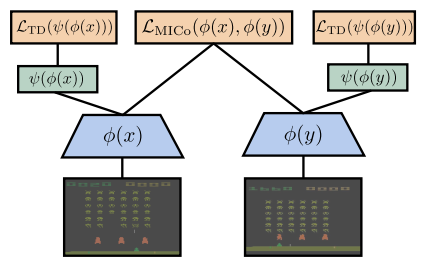
We assume a value-based agent learning an estimate $Q_{\xi,\omega}$ defined by the composition of two function approximators $\psi$ and $\phi$ with parameters $\xi$ and $\omega$, respectively: $Q_{\xi, \omega}(x, \cdot) = \psi_{\xi}(\phi_{\omega}(x))$. We will refer to $\phi_{\omega}(x)$ as the representation of state $x$ and aim to make distances between representations match the MICo distance; we refer to $\psi_{\xi}$ as the value approximator. We define the parameterized representation distance, $U_{\omega}$, as an approximant to $U^{\pi}$: $$U^{\pi}(x, y) \approx U_{\omega}(x, y) := \frac{| \phi_{\omega}(x) |_2 + | \phi_{\omega}(y) |_2 }{2} + \beta \theta(\phi_{\omega}(x), \phi_{\omega}(y))$$ where $\theta(\phi_\omega(x), \phi_\omega(y))$ is the angle between vectors $\phi_\omega(x)$ and $\phi_\omega(y)$ and $\beta$ is a scalar. Our learning target is then $$T^U_{\bar{\omega}}(r_x, x’, r_y, y’) = |r_x - r_y| + \gamma U_{\bar{\omega}}(x’, y’)$$ where $\bar{\omega}$ is a separate copy of the network parameters that are synchronised with $\omega$ at infrequent intervals. This is a common practice that was introduced by Mnih et al., [2015] (and in fact, we use the same update schedule they propose). The loss for this learning target is $$\mathcal{L}_{\text{MICo}}(\omega) = \mathbb{E}_{\langle x, r_x, x’\rangle , \langle y, r_y, y’\rangle}\left[ \left(T^U_{\bar{\omega}}(r_x, x’, r_y, y’) - U_{\omega}(x, y)\right)^2 \right]$$
where $\langle x, r_x, x’\rangle$ and $\langle y, r_y, y’\rangle$ are pairs of transitions sampled from the agent’s replay buffer. We can combine $\mathcal{L}_{\text{MICo}}$ with the temporal-difference loss $\mathcal{L}_{\text{TD}}$ of any value-based agent as $(1-\alpha)\mathcal{L}_{\text{TD}} + \alpha\mathcal{L}_{\text{MICo}}$, where $\alpha \in (0,1)$. Each sampled mini-batch is used for both MICo and TD losses. The figure below illustrates the network architecture used for learning:
Although the loss $\mathcal{L}_{\text{MICo}}$ is designed to learn the MICo diffuse metric $U^\pi$, the values of the metric itself are parametrised through $U_\omega$ defined above, which is constituted by several distinct terms. This appears to leave a question as to how the representations $\phi_\omega(x)$ and $\phi_\omega(y)$, as Euclidean vectors, are related to one another when the MICo loss is minimised. Careful inspection of the form of $U_\omega(x, y)$ shows that the (scaled) angular distance between $\phi_\omega(x)$ and $\phi_\omega(y)$ can be recovered from $U_\omega$ by subtracting the learnt approximations to the self-distances $U^\pi(x, x)$ and $U^\pi(y,y)$, as the figure below illustrates:
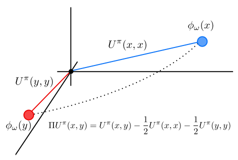
We therefore define the reduced MICo distance $\Pi U^\pi$, which encodes the distances enforced between the representation vectors $\phi_\omega(x)$ and $\phi_\omega(y)$, by: $$\beta \theta(\phi_{\omega}(x) ,\phi_{\omega}(y)) \approx \Pi U^{\pi}(x, y) = U^{\pi}(x, y) - \frac{1}{2}U^{\pi}(x, x) - \frac{1}{2}U^{\pi}(y, y)$$
In the following sections we investigate the following two questions: {\bf (1)} How informative of $V^{\pi}$ is $\Pi U^{\pi}$?; and {\bf (2)} How useful are the features encountered by $\Pi U^{\pi}$ for policy evaluation? We conduct these investigations on tabular environments where we can compute the metrics exactly, which helps clarify the behaviour of our loss when combined with deep networks.
Value bound gaps
Although we have $|V^{\pi}(x) - V^{\pi}(y)| \leq U^{\pi}(x, y)$, we do not, in general, have the same upper bound for $\Pi U^{\pi}(x, y)$ as demonstrated by the following result.
Lemma
There exists an MDP with two states $x$, $y$, and a policy $\pi\in\Pi$ where $|V^{\pi}(x) - V^{\pi}(y)| > \Pi U^{\pi}(x, y)$.
Proof
Consider a single-action MDP with two states ($x$ and $y$) where $y$ is absorbing, $x$ transitions with equal probability to $x$ and $y$, and a reward of $1$ is received only upon taking an action from state $x$.
There is only one policy for this MDP which yields the value function $V(x) \approx 1.8$ and $V(y) = 0$.
The MICo distance gives $U(x, x) \approx 1.06$, $U(x, y) \approx 1.82$, and $U(y, y) = 0$, while the reduced MICo distance yields $\Pi U(x, x) = \Pi U(y, y) = 0$, and $$\Pi U(x, y) \approx 1.29 < |V(x) - V(y)| = 1.8$$
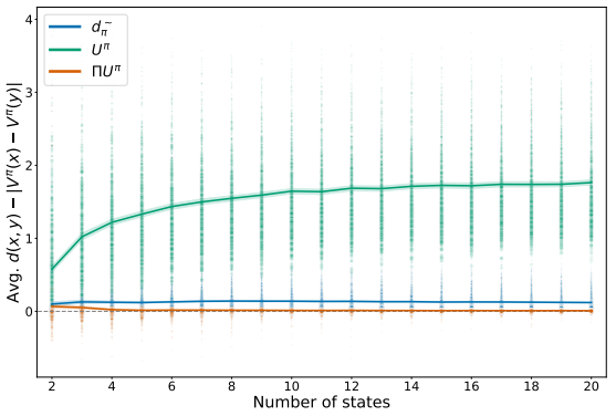
Despite this negative result, it is worth evaluating how often in practice this inequality is violated and by how much, as this directly impacts the utility of this distance for learning representations. To do so in an unbiased manner we make use of Garnet MDPs, which are a class of randomly generated MDPs.
Details of Garnet MDPs
Given a specified number of states $n\_{\mathcal{X}}$ and the number of actions $n\_{\mathcal{A}}$, $\text{Garnet}(n\_{\mathcal{X}}, n\_{\mathcal{A}})$ is generated as follows:- The branching factor $b_{x, a}$ of each transition $P_x^a$ is sampled uniformly from $[1:n_{\mathcal{X}}]$.
- $b_{x, a}$ states are picked uniformly randomly from $\mathcal{X}$ and assigned a random value in $[0, 1]$; these values are then normalized to produce a proper distribution $P_x^a$.
- Each $r_x^a$ is sampled uniformly in $[0, 1]$.
For each $\text{Garnet}(n_{\mathcal{X}}, n_{\mathcal{A}})$ we sample 100 stochastic policies ${\pi_i}$ and compute the average gap: $\frac{1}{100 |\mathcal{X}|^2}\sum_i \sum_{x, y} d(x, y) - |V^{\pi_i}(x) - V^{\pi_i}(y)|$, where $d$ stands for any of the considered metrics. Note we are measuring the signed difference, as we are interested in the frequency with which the upper-bound is violated. As seen in the figure below, our metric does on average provide an upper bound on the difference in values that is also tighter bound than those provided by $U^{\pi}$ and $\pi$-bisimulation. This suggests that the resulting representations remain informative of value similarities, despite the reduction $\Pi$.
State features
In order to investigate the usefuleness of the representations produced by $\Pi U^{\pi}$, we construct state features directly by using the computed distances to project the states into a lower-dimensional space with the UMAP dimensionality reduction algorithm (Note that since UMAP expects a metric, it is ill-defined with the diffuse metric $U^{\pi}$.). We then apply linear regression of the true value function $V^{\pi}$ against the features to compute $\hat{V^{\pi}}$ and measure the average error across the state space. As baselines we compare against random features (RF), Proto Value Functions (PVF) [Mahadevan, 2007], and the features produced by $\pi$-bisimulation. We present our results on three domains in in the figure below, the classic four-rooms GridWorld (left), the mirrored rooms introduced in my paper, and the grid task introduced by Dayan, [1993]:
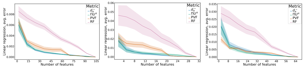
Despite the independent couplings, $\Pi U^{\pi}$ performs on par with $\pi$-bisimulation, which optimizes over all transition probability couplings, suggesting that $\Pi U^{\pi}$ yields good representations.
Empirical evaluation
Having developed a greater understanding of the properties inherent to the representations produced by the MICo loss, we evaluate it on the Arcade Learning Environment. The code necessary to run these experiments is available on GitHub. We will first describe the regular network and training setup for these agents so as to facilitate the description of our loss.
Baseline network and loss description
The networks used by Dopamine for the ALE consist of 3 convolutional layers followed by two fully-connected layers (the output of the networks depends on the agent). We denote the output of the convolutional layers by $\phi_{\omega}$ with parameters $\omega$, and the remaining fully connected layers by $\psi_{\xi}$ with parameters $\xi.$ Thus, given an input state $x$ (e.g. a stack of 4 Atari frames), the output of the network is $Q_{\xi,\omega}(x, \cdot) = \psi_{\xi}(\phi_{\omega}(x))$. Two copies of this network are maintained: an online network and a target network; we will denote the parameters of the target network by $\bar{\xi}$ and $\bar{\omega}$. During learning, the parameters of the online network are updated every 4 environment steps, while the target network parameters are synced with the online network parameters every 8000 environment steps. We refer to the loss used by the various agents considered as $\mathcal{L}_{\text{TD}}$; for example, for DQN this would be: $$\mathcal{L}_{\text{TD}}(\xi, \omega) := \mathbb{E}_{(x, a, r, x’)\sim\mathcal{D}}\left[\rho\left(r + \gamma\max_{a’\in\mathcal{A}}Q_{\bar{\xi},\bar{\omega}}(x’, a’) - Q_{\xi, \omega}(x, a) \right) \right]$$ where $\mathcal{D}$ is a replay buffer with a capacity of 1M transitions, and $\rho$ is the Huber loss.
MICo loss description
We will be applying the MICo loss to $\phi_{\omega}(x)$. As described in \autoref{sec:loss}, we express the distance between two states as: $$U_{\omega}(x, y) = \frac{| \phi_{\omega}(x) |_2 + | \phi_{\bar{\omega}}(y) |_2 }{2} + \beta \theta(\phi_{\omega}(x), \phi_{\bar{\omega}}(y))$$
where $\theta(\phi_\omega(x), \phi_{\bar{\omega}}(y))$ is the angle between vectors $\phi_\omega(x)$ and $\phi_{\bar{\omega}}(y)$ and $\beta$ is a scalar. Note that we are using the target network for the $y$ representations; this was done for learning stability. We used $\beta=0.1$ for the results in the main paper, but present some results with different values of $\beta$ below.
Details on angular distance computation
In order to get a numerically stable operation, we implement the angular distance between representations $\phi_\omega(x)$ and $\phi_\omega(y)$ according to the calculations $$\text{CS}(\phi_\omega(x), \phi_\omega(y)) = \frac{\langle \phi_\omega(x), \phi_\omega(y)\rangle }{|\phi_\omega(x)||\phi_\omega(y)|}$$ $$\theta(\phi_\omega(x), \phi_\omega(y)) = \arctan2\left(\sqrt{1 - \text{CS}(\phi_\omega(x), \phi_\omega(y))^2}, \text{CS}(\phi_\omega(x), \phi_\omega(y))\right)$$
Based on the MICo update operator, our learning target is then (note the target network is used for both representations here): $$T^U_{\bar{\omega}}(r_x, x’, r_y, y’) = |r_x - r_y| + \gamma U_{\bar{\omega}}(x’, y’)$$ and the loss is $$\mathcal{L}_{\text{MICo}}(\omega) = \mathbb{E}_{\langle x, r_x, x’\rangle, \langle y, r_y, y’\rangle\sim\mathcal{D}}\left[ \left(T^U_{\bar{\omega}}(r_x, x’, r_y, y’) - U_{\omega}(x, y)\right)^2 \right]$$
We found it important to use the Huber loss to minimize $\mathcal{L}_{\text{MICo}}$ as this emphasizes greater accuracy for smaller distances as oppoosed to larger distances. We experimented using the MSE loss but found that larger distances tended to overwhelm the optimization process, thereby degrading performance.
As mentioned above, we use the same mini-batch sampled for $\mathcal{L}_{\text{TD}}$ for computing $\mathcal{L}_{\text{MICo}}$. Specifically, we follow the method I introduced for constructing new matrices that allow us to compute the distances between all pairs of sampled states (see code for details on matrix operations).
Our combined loss is then: $$\mathcal{L}_{\alpha}(\xi, \omega) = (1-\alpha)\mathcal{L}_{\text{TD}}(\xi, \omega) + \alpha\mathcal{L}_{\text{MICo}}(\omega)$$
Results
ALE experiments
We added the MICo loss to all the JAX agents provided in the Dopamine library. For all experiments we used the hyperparameter settings provided with Dopamine. We found that a value of $\alpha=0.5$ worked well with quantile-based agents (QR-DQN, IQN, and M-IQN), while a value of $\alpha=0.01$ worked well with DQN and Rainbow. We hypothesise that the difference in scale of the quantile, categorical, and non-distributional loss functions concerned leads to these distinct values of $\alpha$ performing well. We found it important to use the Huber loss to minimize $\mathcal{L}_{\text{MICo}}$ as this emphasizes greater accuracy for smaller distances as oppoosed to larger distances. We experimented using the MSE loss but found that larger distances tended to overwhelm the optimization process, thereby degrading performance. We evaluated on all 60 Atari 2600 games over 5 seeds.
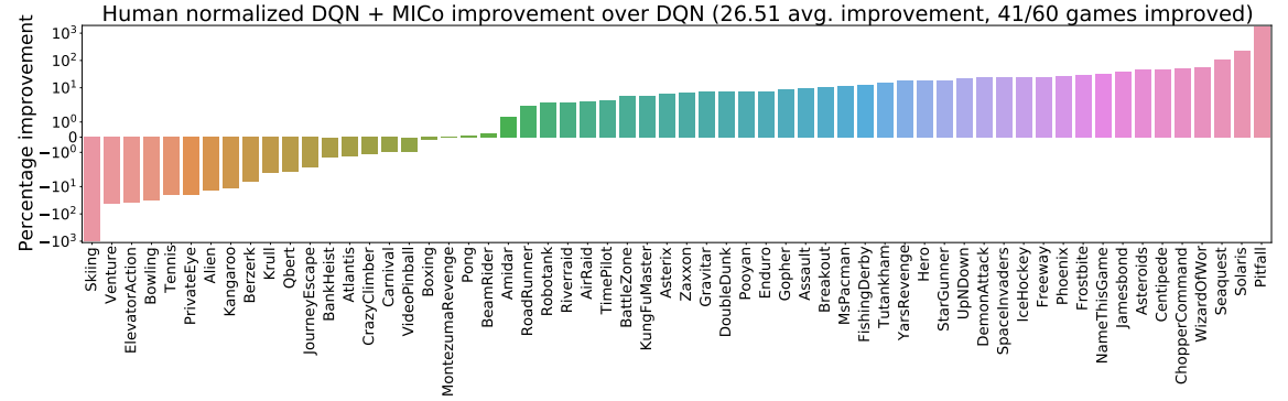
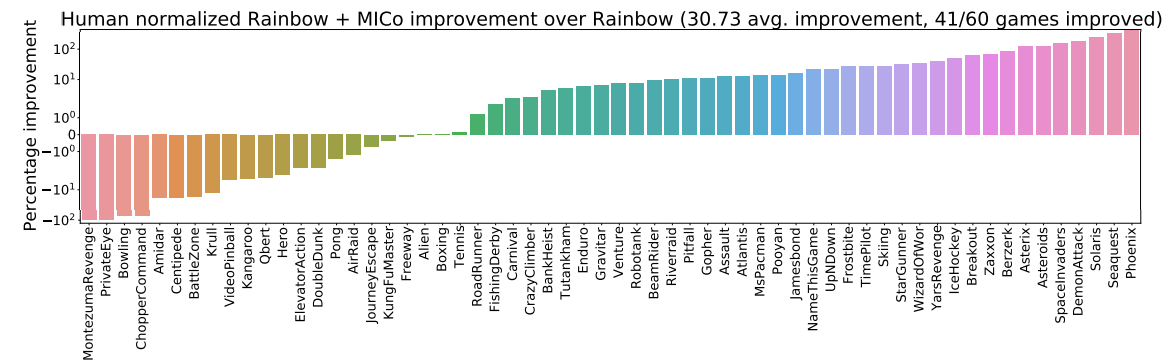
We begin by presenting the improvements achieved for each agent in the bar plots below:
- DQN, using mean squared error loss to minimize $\mathcal{L}_{\text{TD}}$ for DQN (as suggested in our recent Revisiting Rainbow paper)
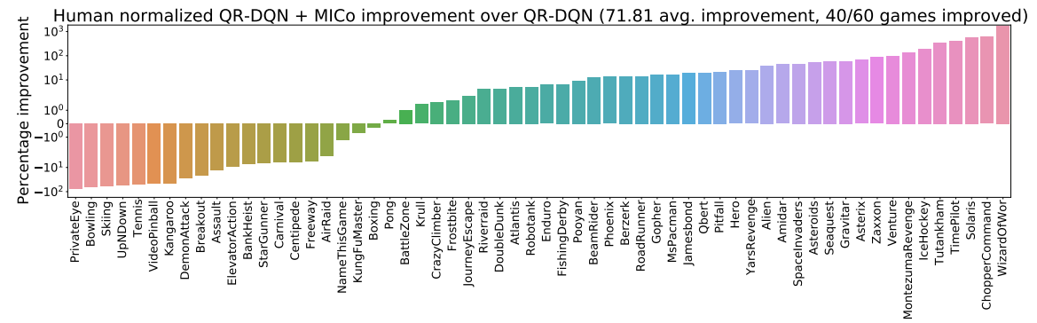
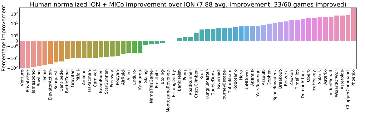
- M-IQN; given that the authors had implemented their agent in TensorFlow (whereas our agents are in JAX), we have reimplemented M-IQN in JAX and run 5 independent runs (in contrast to the 3 run by the authors).
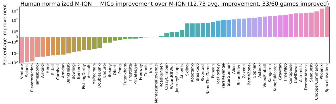
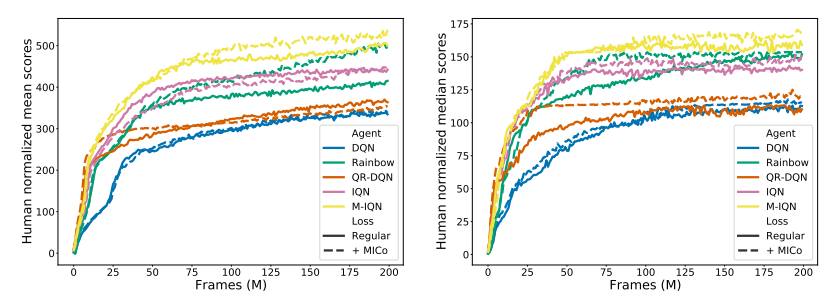
The figure below presents the aggregate normalized performance across all games; as can be seen, our loss is able to provide good improvements over the agents they are based on, suggesting that the MICo loss can help learn better representations for control.
DM-Control experiments
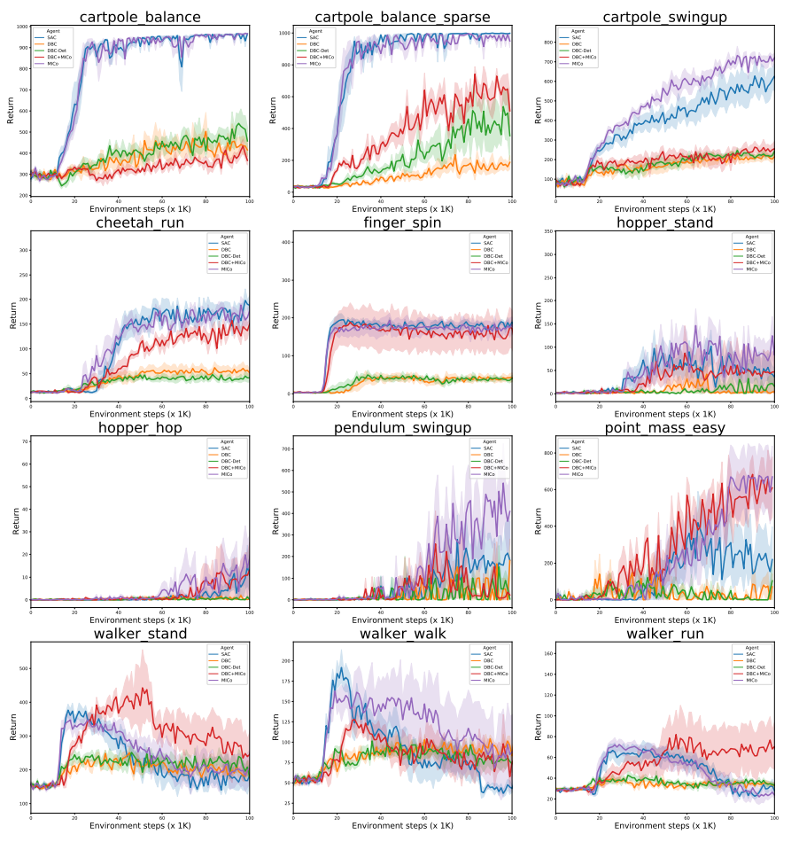
Additionally, we evaluated the MICo loss on twelve of the DM-Control suite from pixels environments. As a base agent we used Soft Actor-Critic (SAC) from Haarnoja et al. with the convolutional auto-encoder described by Yarats et al.. We applied the MICo loss on the output of the auto-encoder (with $\alpha=1e-5$) and maintained all other parameters untouched. Recently, Zhang et al. introduced DBC, which learns a dynamics and reward model on the output of the auto-encoder; their bisimulation loss uses the learned dynamics model in the computation of the Kantorovich distance between the next state transitions. We consider two variants of their algorithm: one which learns a stochastic dynamics model (DBC), and one which learns a deterministic dynamics model (DBC-Det). We replaced their bisimulation loss with the MICo loss (which, importantly, does not require a dynamics model) and kept all other parameters untouched. As the figure at the top of post illustrates, the best performance is achieved with SAC augmented with the MICo loss; additionally, replacing the bisimulation loss of DBC with the MICo loss is able to recover the performance of DBC to match that of SAC.
Here we present the learning curves for all the DM-Control environments run.
Conclusion
In this paper, we have introduced the MICo distance, a notion of state similarity that can be learnt at scale and from samples. We have studied the theoretical properties of MICo, and proposed a new loss to make the non-zero self-distances of this diffuse metric compatible with function approximation, combining it with a variety of deep RL agents to obtain strong performance on the Arcade Learning Environment. In contrast to auxiliary losses that implicitly shape an agent’s representation, MICo directly modifies the features learnt by a deep RL agent; our results indicate that this helps improve performance. To the best of our knowledge, this is the first time directly shaping the representation of RL agents has been successfully applied at scale. We believe this represents an interesting new approach to representation learning in RL; continuing to develop theory, algorithms and implementations for direct representation shaping in deep RL is an important and promising direction for future work.
Acknowledgements
The authors would like to thank Gheorghe Comanici, Rishabh Agarwal, Nino Vieillard, and Matthieu Geist for their valuable feedback on the paper and experiments. Pablo Samuel Castro would like to thank Roman Novak and Jascha Sohl-Dickstein for their help in getting angular distances to work stably! Finally, the authors would like to thank the reviewers (both ICML'21 and NeurIPS'21) for helping make this paper better.
comments powered by Disqus