In Defense of Atari - the ALE is not 'solved'!

This post is based on a talk I gave at the AutoRL workshop in ICML 2024, which unfortunately was not recorded.

Introduction

Reinforcement Learning (RL) has been used successfully in a number of challenging tasks, such as beating world champions at Go, controlling tokamak plasmas for nuclear fusion, optimized chip placement, and controlling stratospheric balloons. All these successes have leveraged years of research and expertise and, importantly, rely on the combination of RL algorithms with deep neural networks (as proposed in the seminal DQN paper).

The use of deep networks has become the norm for most (non-theoretical) RL research papers published. One very common structure for these types of papers is the following:

Motivate the problem
Define the baseline algorithm on which the work will be building on
Present some theoretical result (which almost always is limited to linear function approximators)
Introduce the paper’s fancy new idea, building on the theory and adapted to neural nets (where the theory no longer holds)
Evaluate on a common benchmark suite (like the Arcade Learning Environment).
Aggregate scores from the suite and generate a plot that shows the new algorithm is above the baseline
Profit!

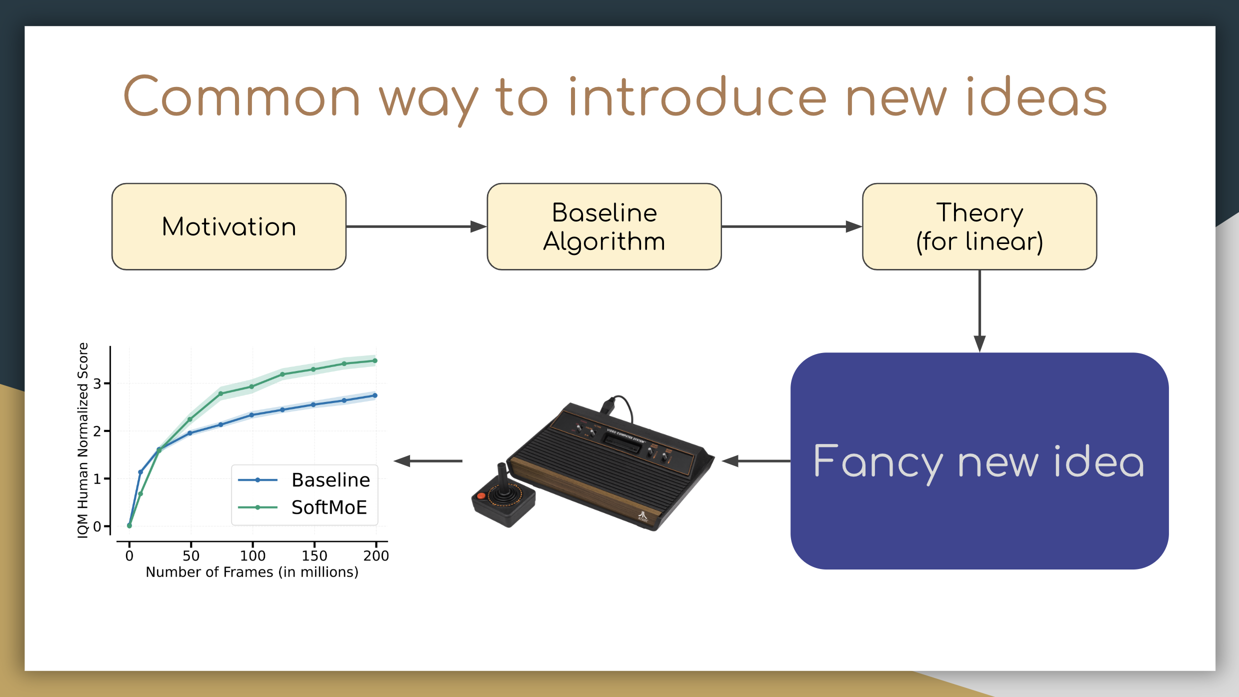
The Arcade Learning Environment has been one of the most common benchmarks on which to play this “profit” game, and we have developed many algorithms that play most Atari games at superhuman levels. This has led many in the community to profess things like:

“Atari is solved”
“Research on the ALE is no longer interesting”
“Interesting paper, but I will keep my score of reject because the authors shouldn’t focus on Atari results”

While I’m always in favour of more experiments, I don’t believe any of the previous statements to be true; indeed, I believe the ALE can be an incredibly useful research platform, as long as we’re asking the right questions. I’ll try to argue this in the rest of this blogpost.

RL in the real world

What happens if one wants to take the latest-and-greatest RL algorithm to use in a real-world device? Can one just plug in this RL algorithm into a robot vacuum cleaner and have it avoid getting stuck on things (as mine always does)?

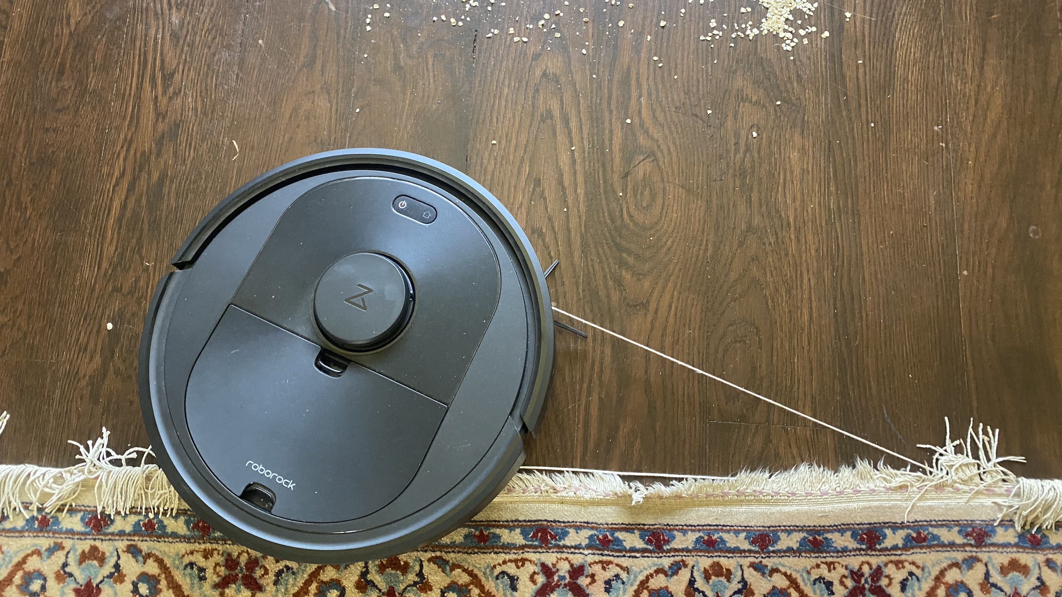
The answer is almost always no! In fact, none of the success stories listed above used an out-of-the-box method; they all required a team of RL researchers in order to make them work properly. Of course, one of the big reasons for the failure of “direct transfer” is that the environments are different (i.e. different transition and reward dynamics, different observations, different action spaces, etc.). In addition to this comes all the many variatiinos we can make to the algorithms, including:

Choice of base algorithm
- Do we use value-based? Discrete? Off-policy? …
Choice of network
- What architecture do we use? Do we use normalization? What activations and initializations? …
Optimization choices
- What optimizer? What learning rate? Do we use a schedule? …
Replay buffer choices
- What capacity? What sampling strategy do we use? What batch size do we use for sampling? …
RL components
- What discount factor do we use? What update period? Do we use multi-step returns? Lambda returns? Importance sampling? …
…

Measuring progress

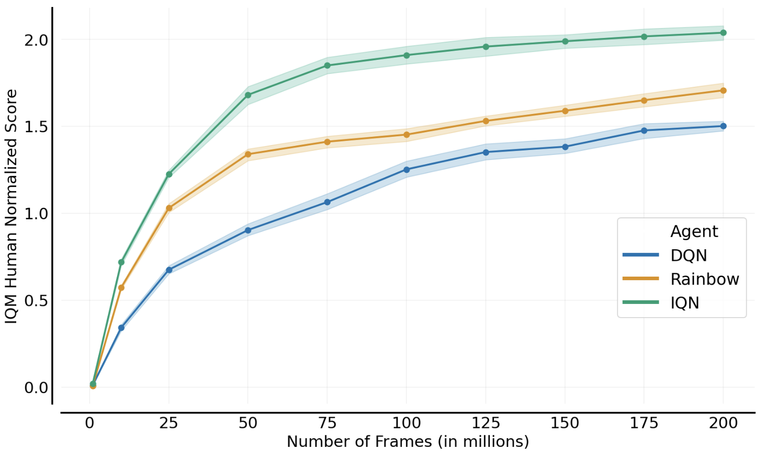
As seen above, there are a lot of choices to be made. Yet, despite this, we still see progress when we directly build on prior work? In the plot below (generated with Dopamine, we can see the progress from DQN to Rainbow to IQN, as evaluated on the ALE.

Is aggregate progress enough?

The plot above is aggregating multiple runs across multiple games using human-normalized Interquartile Mean (as we proposed in our paper), which is a common practice in RL research papers. However, if we look at the training curves for individual games, we can see that the ordering is inconsistent.

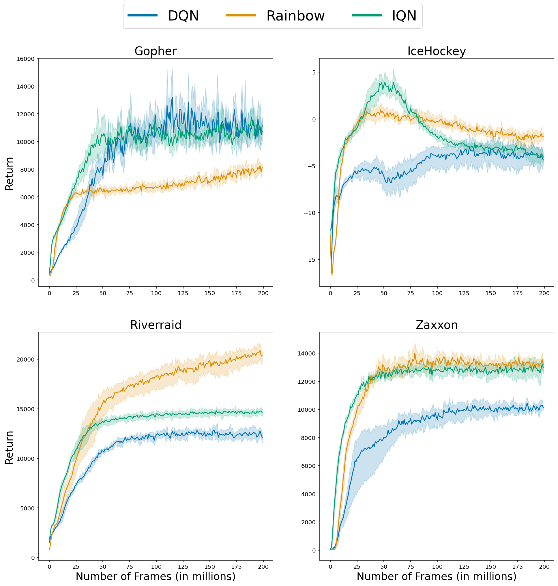
This inconsistency is present in pretty much any algorithm comparison out there! Thus, although aggregate results are good for providing a concise summary of performance,

aggregate results can hide important per-game differences between algorithms!

Are we always making progress?

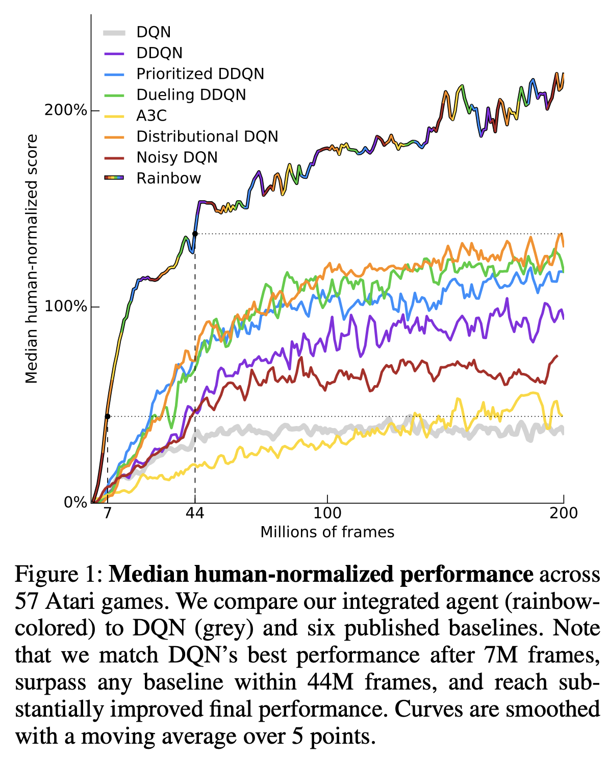
This section tells the story of how the DER agent came about. In 2018, Hessel et al. introduced the Rainbow algorithm, which combined six recent algorithmic advances into one “mega” agent, which was state-of-the-art for the time.

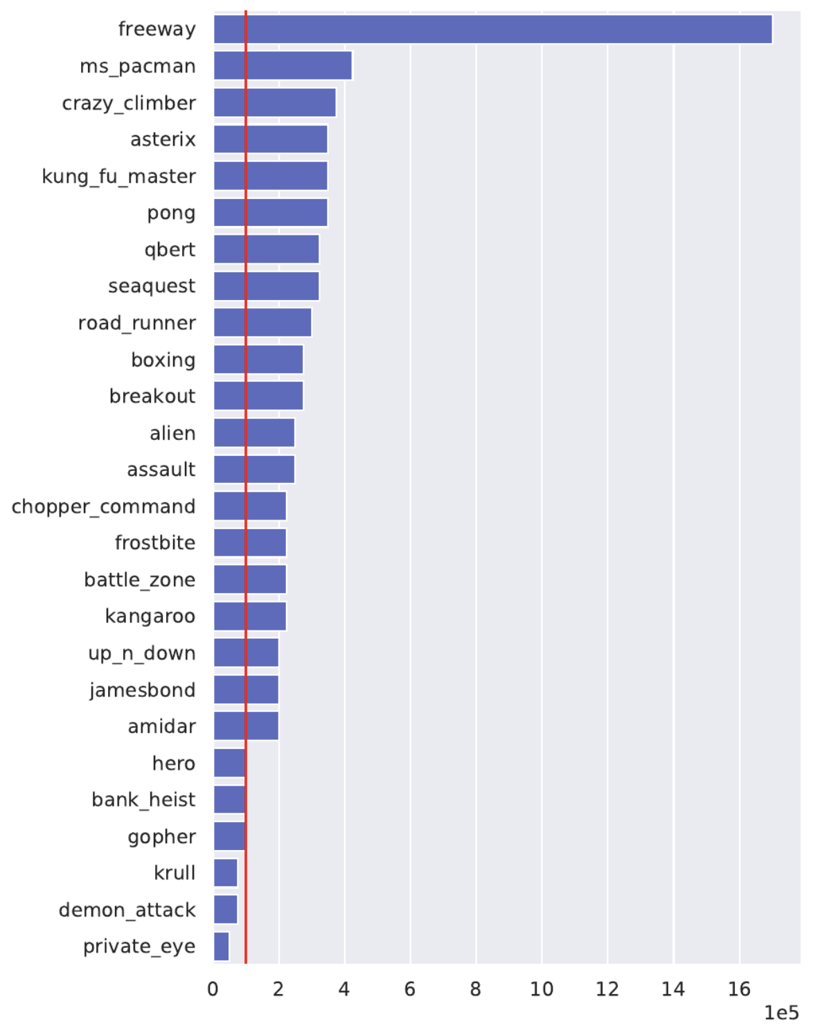
In 2020, Kaiser et al. introduced SimPLe, a model-based method that aimed for extreme sample efficiency. As discussed in a recent blog post, the standard 200M environment frames on which DQN and Rainbow are evaluated is quite a lot of environment interactions! Kaiser et al. proposed a new benchmark which only allowed 100k agent decisions (equivalent to 400k environment frames, due to frame skipping); this benchmark was dubbed the Atari 100k benchmark and included only a subset of 26 games on which progress was achievable with 100k agent decisions. In the figure below, the authors plotted the number of agent interactions needed by Rainbow in order to match the performance of their SimPLe with only 100k interactions (red line). Clearly SimPLe is much more sample efficient!

The story doesn’t end there, though. Some of the authors of the original Rainbow paper published a paper where they optimized the hyper-parameters of Rainbow for the Atari 100k benchmark without changing anything else, and demonstrated that their DER (Data-Efficient Rainbow) outperformed SimPLe on the Atari 100k benchmark!

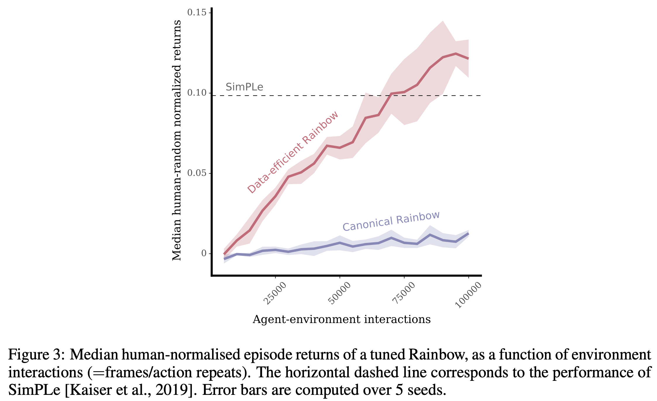
One could argue that the hyper-parameters of Rainbow were overly-tuned to the 200M benchmark, while the hyper-parameters of DER were overly-tuned to the 100k benchmark. More importantly, what this story highlights is that, despite careful evaluation it is quite likely that a new method will not work as intended when deployed on a different environment from which it was trained on, and that a significant amount of hyper-parameter tuning will be necessary. The important takeaway from this story is that:

you cannot compare against a baseline in a new benchmark unless you also do hyper-parameter optimization for the baseline in the new benchmark!

Amusingly, even though DER was developed after SimPLe, it was officially published before it (the DER authors were likely basing their comparison on a pre-print of the SimPLE paper).

When do hyper-parameter settings transfer?

The story above suggests that hyper-parameter configurations are specific to the setting on which they are evaluated. In a recent RLC paper we investigated whether hyper-parameter configurations transfer:

Across agents (between DER and DrQ($\epsilon$))
Across data regimes (between 100k and 10M environment interactions)
Across environments (using the 26 environments from the Atari 100k benchmark)

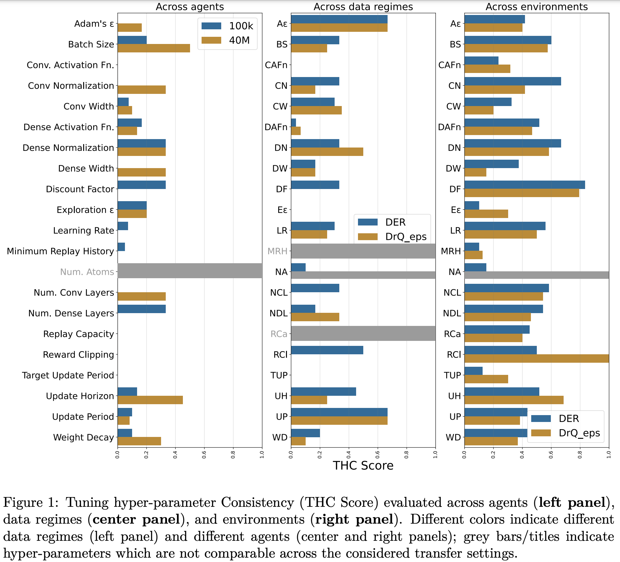
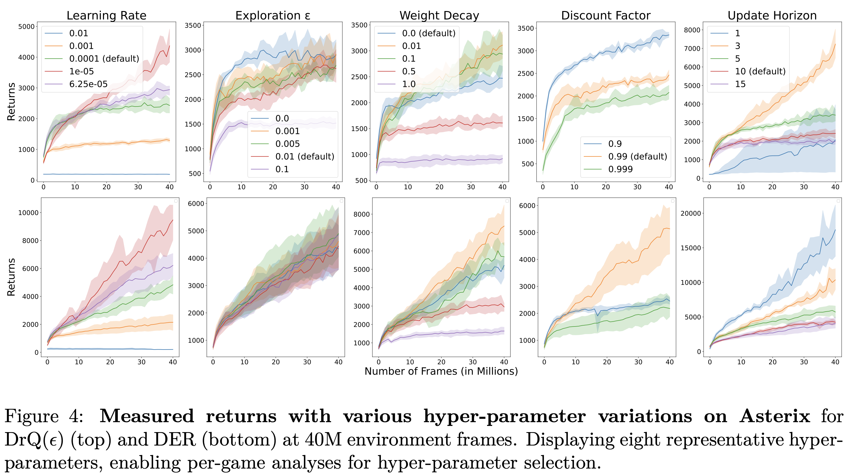
To do this, we investigated 12 hyper-parameters with different values for 2 agents (DER and DrQ($\epsilon$) over 26 environments, evaluated for both 100k and 10M agent interactions, each for 5 seeds, resulting in a total of over 108k independent training runs. This results in an overwhelming number of plots to digest, so we provided a website to facilitate navigation of the full set of results. Given a set of hyper-parameter values to choose from, we were interesting in determining whether the ranking of those values remains consistent across the three forms of transfer mentioned above. We defined the THC metric (see paper for details), which provides, for each hyper-parameter, an aggregate quantification of its transferability (higher values means less transferability):

(Mostly) across agents

In the figure above we can see that when evaluating transferability across agents, we generally have low THC scores, which indicates that hyper-parameter orderings are mostly consistent. Inspecting a few individual games confirms this, where DrQ($\epsilon$) is in the top row and DER in the bottom row.

Not across data regimes

When we inspect the ordering of hyper-parameter values when evaluated on 100k versus 10M agent interactions we get far less consistency, as can ben seen by higher THC scores above and the figure below, where the ordering basically flips from one regime to the next!

Not really across environments

The ranking of hyper-parameter values does not really remain consistent across environments, as evidenced by the high THC scores above. If we inspect the performance of DrQ($\epsilon$) while varying batch size on a few games, we can see that the rankings can sometimes be completely flipped (compare Asterix and Gopher versus BattleZone and Kangaroo):

Wakeup call!

The above results should be a wakeup call:

If we can’t get our agents to work reliably in Atari, what hope have we for other real-world complex systems?

Why the ALE is still a great benchmark for RL research

The last statement can be phrased differently: the ALE is a great benchmark for developing methods that are consistent across different training regimes, robust to varying hyper-parameters, without sacrificing performance. Here are some more reasons why it’s (still) a great benchmark for general RL research.

Diversity of “non-biased” environments

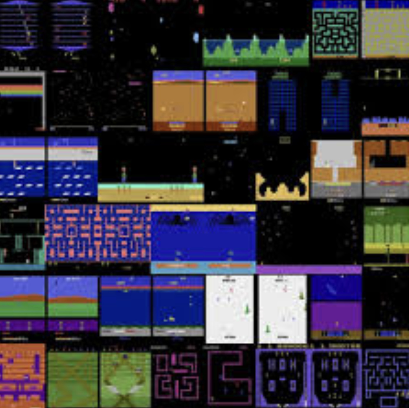
The ALE suites consists of over 57 games (I normally run with 60) which vary in difficulty, reward sparsity, observational complexity, and transition dynamics. Importantly, these games were developed by professional game designers for human enjoyment, and not by RL researchers for RL research. This mitigates experimenter bias which is unfortunately present in many of the environment suites that have been developed specifically for RL research.

Variety of difficulty modes

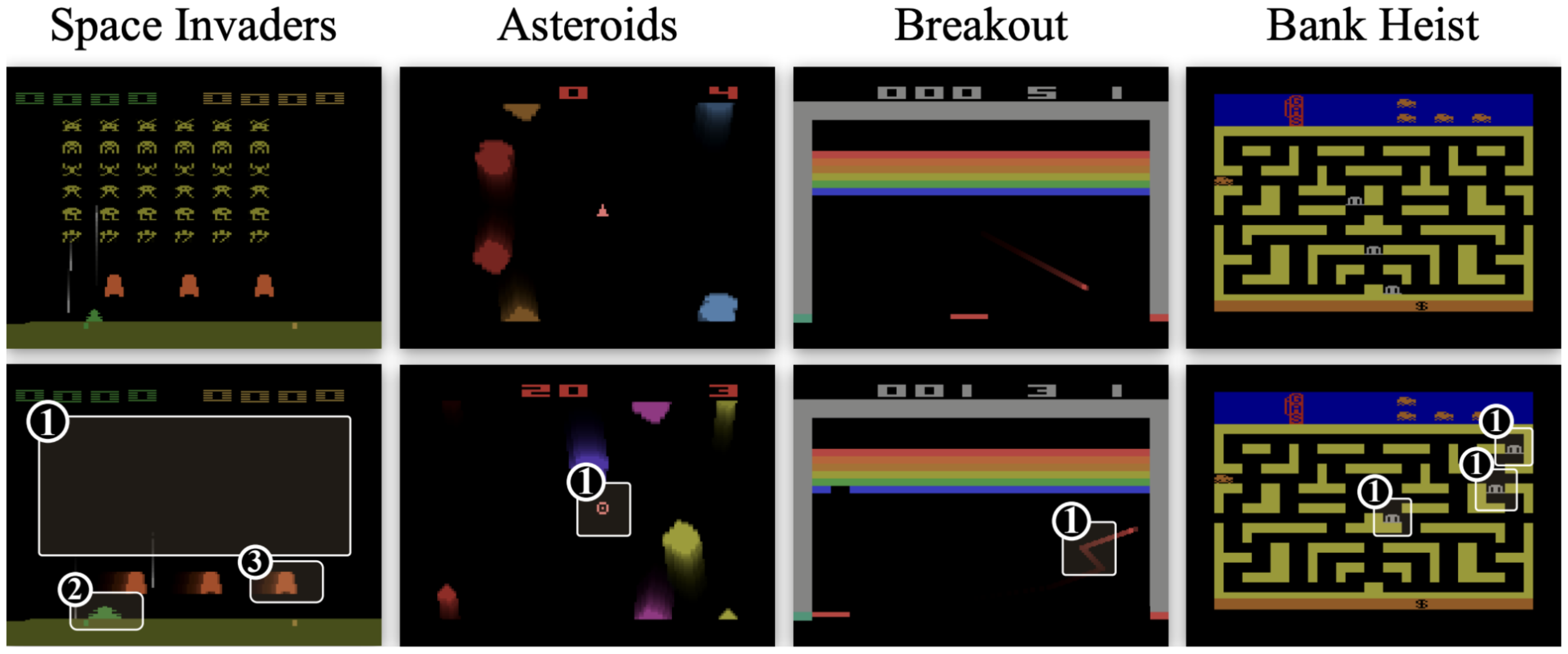
Many of these games also include a variety of difficulty modes which allows us to carefully investigate the generalization capabilities of our agents (read more about modes here, and here).

Deterministic versus stochastic variants

The Atari games in the ALE were originally deterministic, but Machado et al. introduced “sticky actions”, which causes actions to repeat (or “stick”) with some probability, thereby rendering the environment transitions stochastic. This can make games more/less difficult, and can avoid trivial open-loop policy solutions.

Discrete versus continuous control

Since its introduction, the ALE has been a suite of discrete action environments; however, the original joystick is an analogue controller! In our latest NeurIPS'24 paper, we introduce CALE, the Continuous ALE, which enables continuous actions for the ALE. Rather than having 9 discrete positions for each joystick position (see top left circle in figure below), we parameterize the actions via three continuous dimensions: two for polar coordinates and one for the “fire” button. Depending on a sensitivity threshold $\tau$, the joystick position still triggers one of the 9 discrete position events.

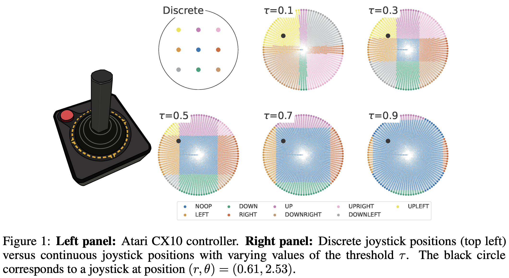
Discrete versus continuous actions in the CALE

After those events are triggered, the emulator is exactly the same for both the ALE and the CALE, which means that:

The only difference between the ALE and the CALE is the input action space!

The advantage of this is that we have a much more direct way to compare discrete- and continuous-action agents, without any “actor head” modifications! We trained SAC and PPO on the CALE and compared them against DQN and SAC-D (a discrete version of SAC proposed here).

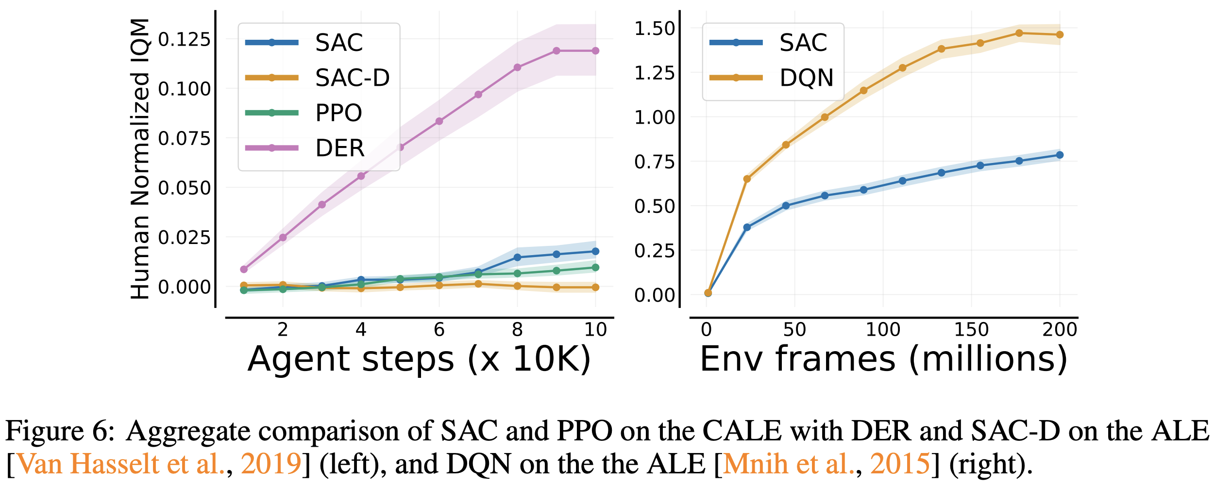
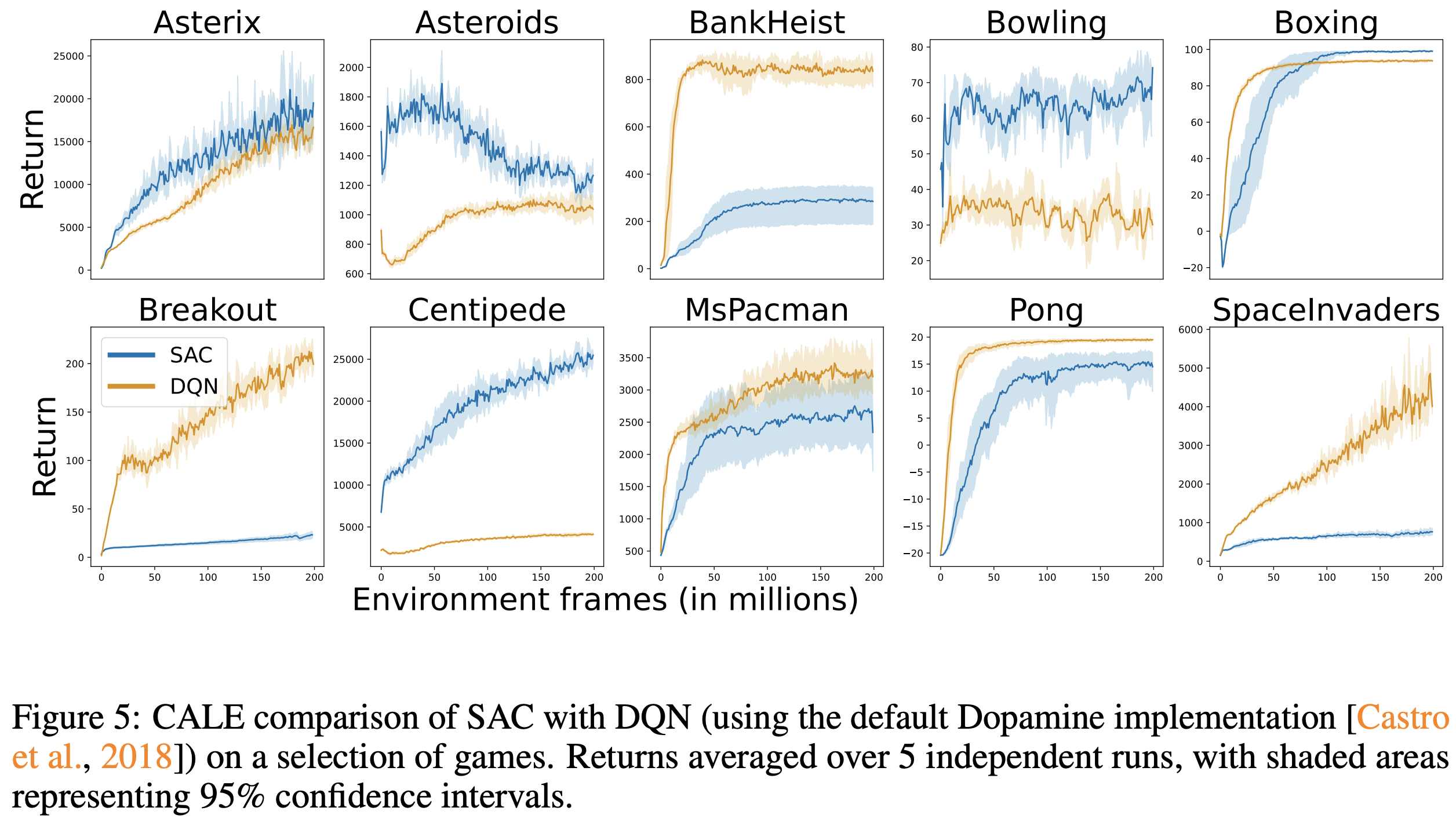
The fact that the continuous control agents (PPO and SAC) drastically under-perform their discrete counterparts is not entirely surprising, as they have not (yet) been optimized for the CALE. What is interesting to observe is that the dominance of DQN over SAC is not uniform across games, which is very much consistent with the discussions above:

Other extensions

Aside from the above, there have been many interesting extensions to the ALE, a few of which I list below:

Well-established benchmark

Of course, an important point of the ALE is that it is already a well-establishedf and well-understood benchmark, which makes it easier for readers (including reviewers) to process results.

Use the ALE, but use it properly!

I hope this post has convinced you of why the ALE (and its extensions) is still a great benchmark for RL research. When you’re reviewing papers and want to dock points for focusing on the ALE, please keep this post in mind. If you’re an author and a reviewer is giving you grief about focusing on Atari, feel free to point them to this post! Of course, this assumes that you’re asking the right questions. Here are some tips to (hopefully) help in this respect.

Stop focusing only on aggregate plots

Keep track of games where your method improves and those where it degrades

Are there patterns?
Does ordering change with different hparam choices?
Discuss these in your work!

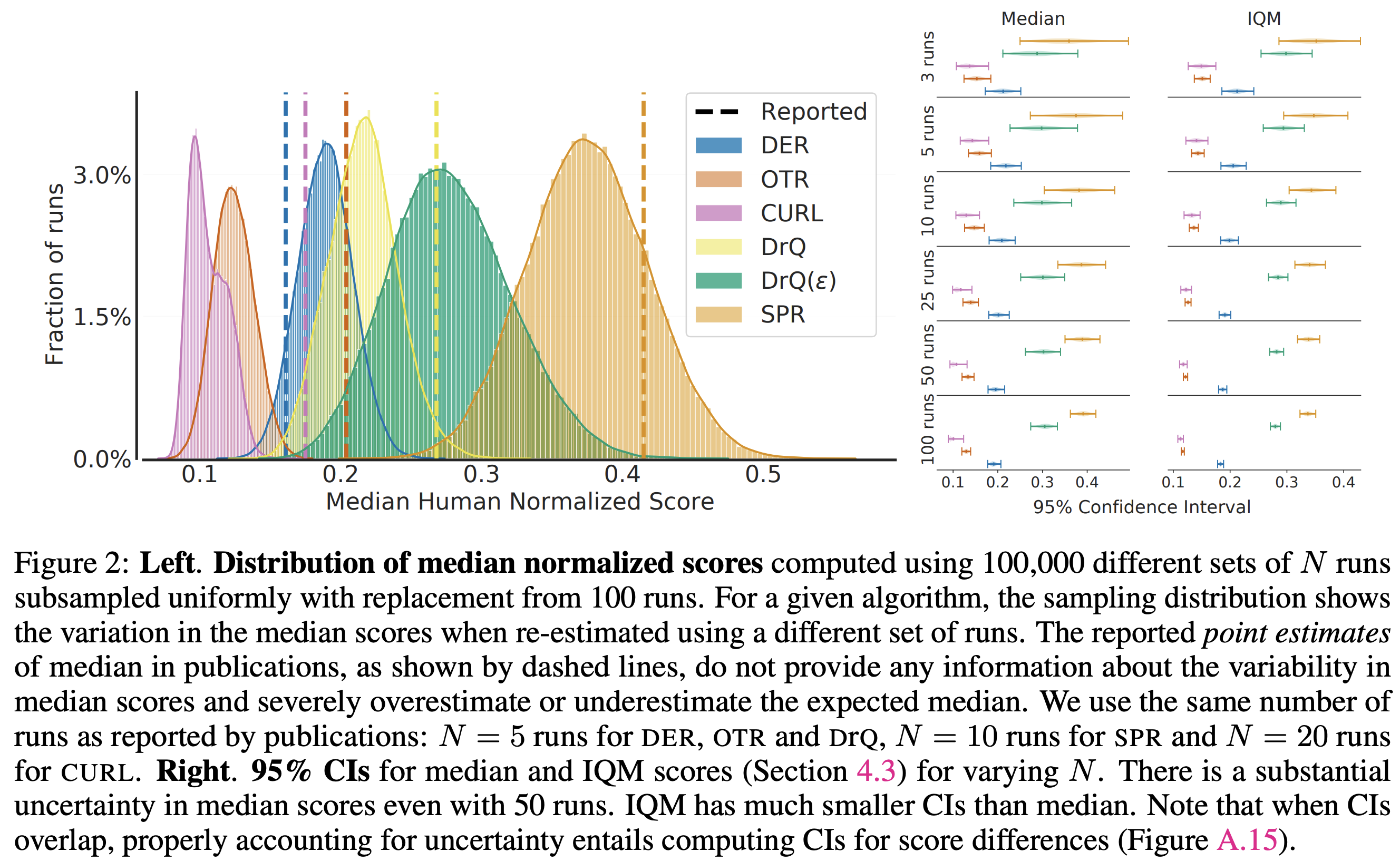
Measure distribution of scores

If you can, report a distribution of scores rather than a single statistic, and consider measure the consistency of your results with bootstrapping (as we did in our paper).

Don’t exclude games

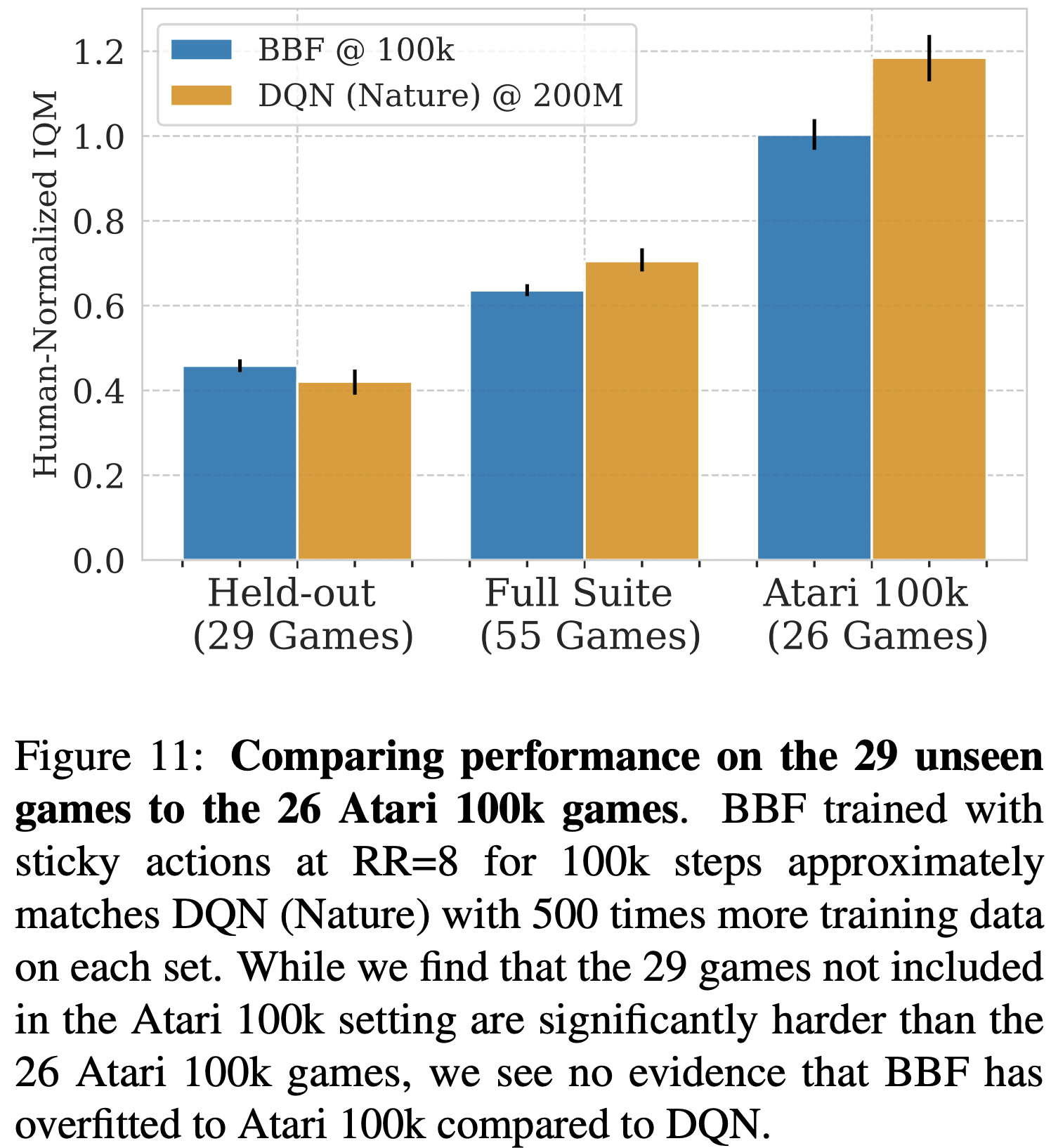
For computational reasons, many works often focus their analyses on a subset of games. If you have the compute, run at least one experiment on the set of all games as this helps evaluate the generalizability of the claims. For example, in our BBF paper we were mostly focused on the 26 Atari 100k games, but did run comparisons on the remaining games.

Run for longer / shorter

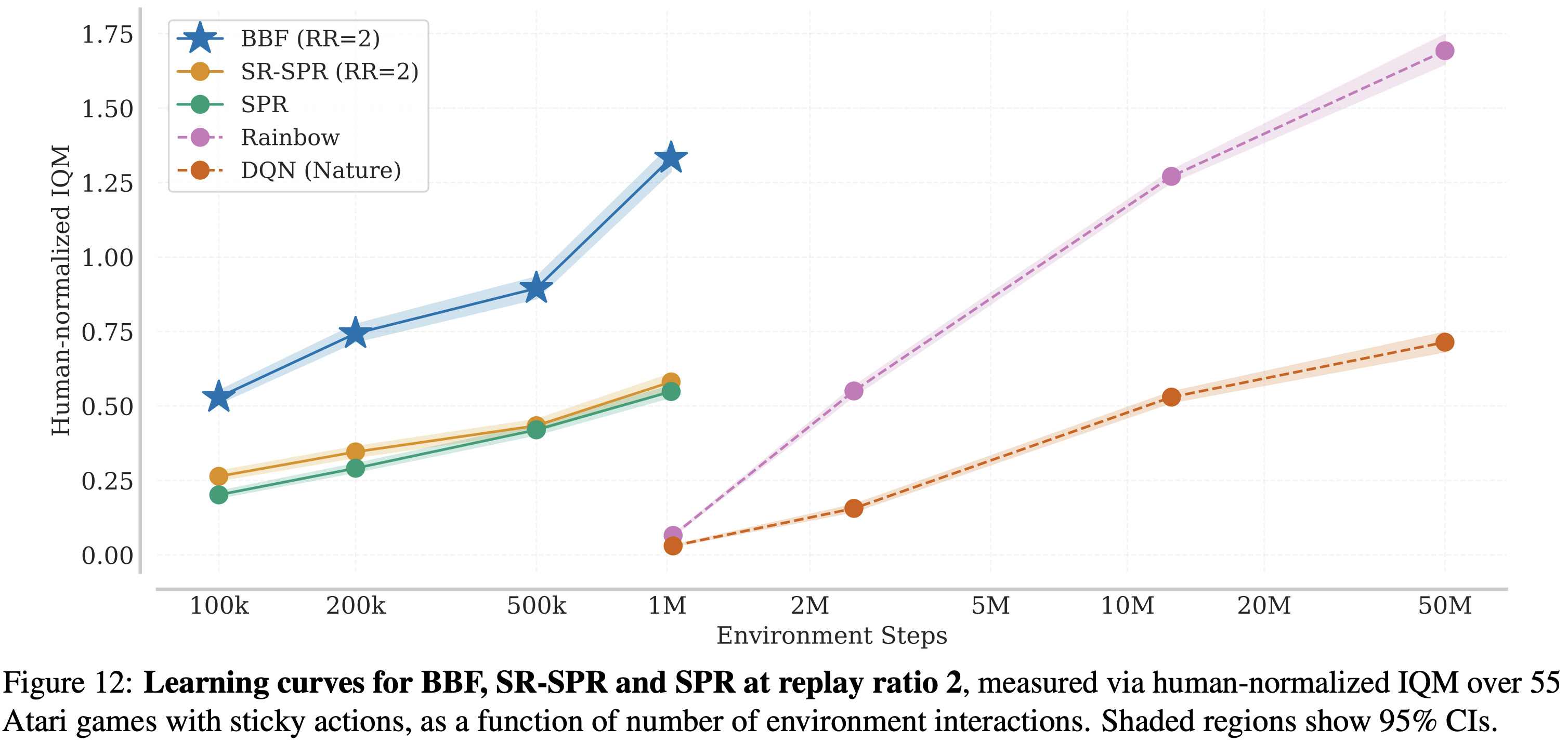
Try to run for different training lengths. As discussed above, changing the data regimes can have a dramatic effect on reported performance! This is something discussed in the excellent Empirical Design in Reinforcement Learning, and something we did in our BBF paper:

Better characterization of games

The huge variance we see across games demonstrates that we lack good, quantifiable, characterizations for these games. Most characterizations have been rather high-level and manually crafted (e.g. “sparse reward” games), with the Atari-5 paper providing a bit more granularity:

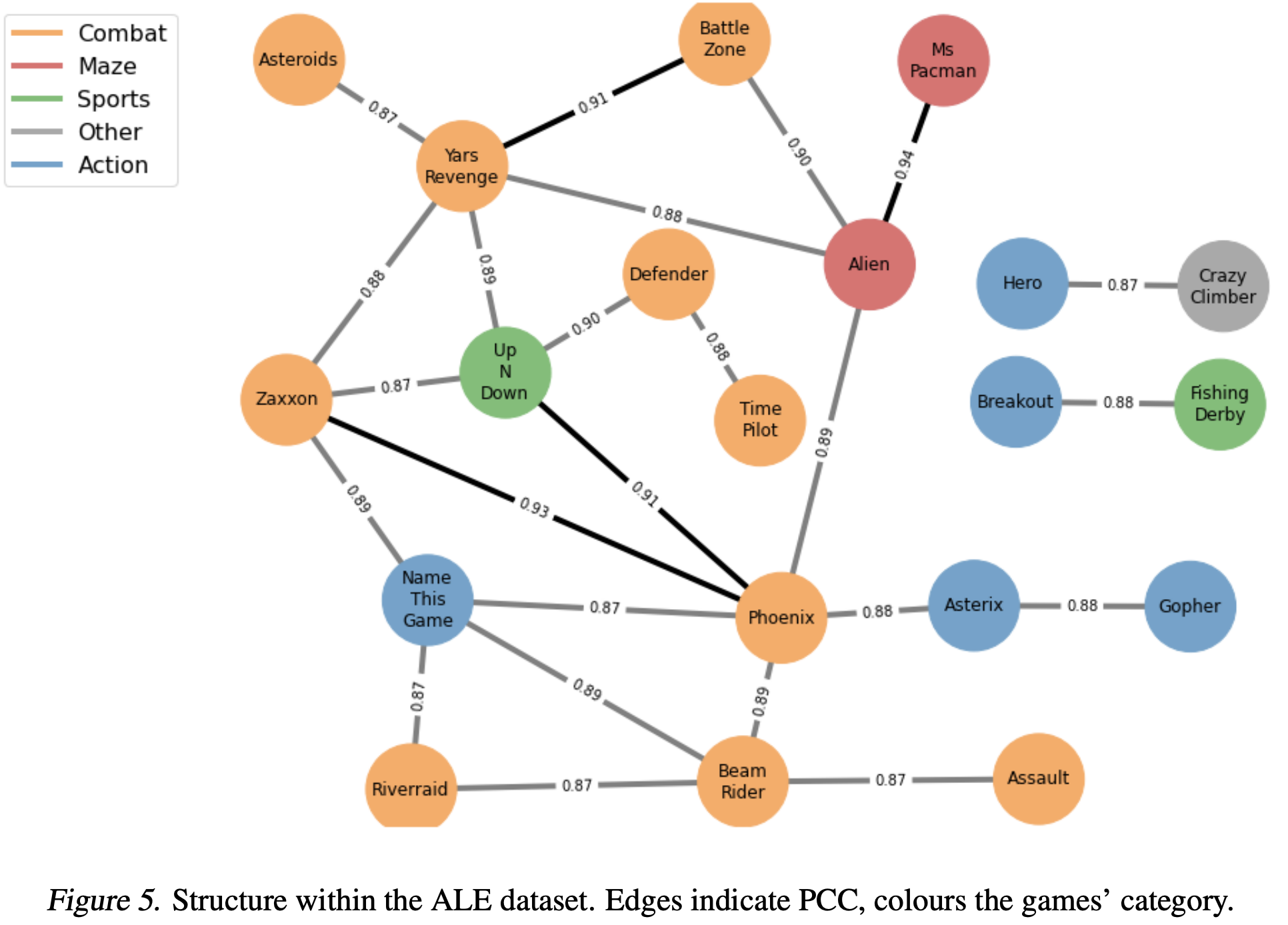
Ideally we would have a rich enough characterizations of the various games (that are useful for general environments) that enable automatically adjusting hyper-parameter settings for each environment.

Conclusion

If our only goal is to “play Atari games really really well”, then maybe we’re done. But that was never the point of the ALE, it was always meant as a research platform. We should be striving to develop methods that are reliable and transferable, and this requires going beyond pure “SotA-chasing”, and even beyond cumulative returns, and conducting more thorough and “nitty-gritty” analyses to get a better sense of what makes deep RL agents tick. I think we should asking ourselves why our algorithms learn/behave the way they do, rather than trying to squeeze out some extra IQM points to claim SotA.

The ALE is an extremely valuable resource in our mission to develop more generally capable agents, as long as you ask the right questions and use it properly!

P.S. If you want to learn about the history of how the originally Atari 2600 console was developed, I highly recommend the book Racing the Beam.

Pablo Samuel Castro