Losses, Dissonances, and Distortions

Exploiting the creative possibilities of the numerical signals obtained during the training of a machine learning model.

I will be presenting this paper at the 5th Machine Learning for Creativity and Design Workshop at NeurIPS 2021.

The code is available here.

You can see an “expainody” video here:

Introduction

In recent years, there has been a growing interest in using machine learning models for creative purposes. In most cases, this is with the use of large generative models which, as their name implies, can generate high-quality and realistic outputs in music, images, text, and others. The standard approach for artistic creation using these models is to take a pre-trained model (or set of models) and use them for producing output. The artist directs the model’s generation by ``navigating’’ the latent space, fine-tuning the trained parameters, or using the model’s output to steer another generative process (e.g. two examples).

At a high-level what all these approaches are doing is converting the numerical signal of a machine learning model’s output into art, whether implicitly or explicitly. However, in most (if not all) cases they only do so after the initial model has been trained. This is somewhat unfortunate, as there are plenty of numerical signals available during the training process, such as the loss and gradient values, that can be used for creative purposes.

In this work I study using the losses and gradients obtained during the training of a simple function approximator as a mechanism for creating musical dissonance and visual distortion in a solo piano performance setting. These dissonances and distortions become part of an artistic performance not just by affecting the visualizations, but also by affecting the artistic musical performance. The system is designed such that the performer can in turn affect the training process itself, thereby creating a closed feedback loop between two processes: the training of a machine learning model and the performance of an improvised piano piece.

Components

Losses and gradients

Let $f_\theta:X\rightarrow Y$ denote a function parameterized by a $d$-dimensional vector of weights $\theta\in\mathbb{R}^d$ that aims to approximate a “true” function $f:X\rightarrow Y$. We improve the approximation by updating the parameters $\theta$ so as to minimize a loss function $\mathcal{L}(f_\theta, f)\rightarrow\mathbb{R}$. This is typically done using gradient descent, where we use the derivative (or gradient) of the loss function to update the parameters: $\theta \leftarrow \theta - \alpha \nabla \mathcal{L}(f_\theta, f)$, where $\alpha$ is a learning rate. If set properly, this process will result in $\mathcal{L}\rightarrow 0$.

Thus, at every iteration of the learning process we have $d+1$ values at our disposal: the $d$ partial gradients from $\nabla\mathcal{L}$ and the loss itself. In the next sections I will describe how I use these values as part of a performance, but of course there are an infinitude of ways that artists can incorporate these as part of their work.

Cubics

In order for the learning dynamics to be clearly observed during the performance, it is preferable that the learning process is able to converge relatively quickly. For this reason I chose two relatively simple functions to learn: Cubic polynomials and Lissajous knots.

The polynomials are single-valued functions $f_{a,b,c,d}:\mathbb{R}\rightarrow\mathbb{R}$:

$$f_{{\bf a,b,c,d}}(x) = ax^3 + bx^2 + cx + d$$

The parameters $\theta$ of the learned function aim to approach the true values of $a$, $b$, $c$, and $d$. We use the mean-squared error loss:

$$ \mathbb{E}_x\left[\sqrt{\left(f_{a,b,c,d}(x) - f_{\theta}(x)\right)^2}\right] $$

You can play with the following widget to see learning cubics in action:

numPoints: iterations: Regenerate Learn!

Lissajous knots

Lissajous knots are multi-valued functions $g_{n_x,n_y,n_z,a,b,c}:\mathbb{R}\rightarrow\mathbb{R}^3$, where $n_x$, $n_y$, and $n_z$ are integers:

$$g_{n_x,n_y,n_z,{\bf a,b,c}}(t) = \langle cos(n_x t + a), cos(n_y t + b), cos(n_z t + c) \rangle $$

The parameters $\theta$ of the learned function aim to approach the true values of $a$, $b$, and $c$ (e.g. the integer-parameters are not learned). We again use the mean-squared error loss:

$$\mathbb{E}_t\left[\sqrt{\left(g_{n_x,n_y,n_z,a,b,c}(t) - g_\theta\right(t))^2}\right]$$

Dissonances

Music is made of the combination of individual {\em notes} played on a variety of instruments. Each note is actually a combination of a number of pitches or frequencies: the {\em fundamental frequency}\footnote{This is typically what is referred to as “the pitch” of a played note.}; and a series of {\em overtone frequencies}, that are pitches at higher frequencies than the fundamental. A well-tuned instrument will have overtones that are {\em multiples} of the fundamental frequency (and in this case, these are called harmonics). For example, a well-tuned A note may have the following frequencies (one fundamental and three overtones): $\lbrace 440, 880, 1320, 1760 \rbrace$. If we detune the overtones by an amount proportional to the loss: $\lbrace 440, 880 (1 + \mathcal{L}), 1320 (1 + \mathcal{L}), 1760 (1 + \mathcal{L}) \rbrace$, then what we will hear throughout the learning process is the sound “converging” to its well-tuned state, starting from a detuned state (play with an example here.

Distortions

In addition to creating dissonance, we can create visual distortions using the partial gradients of $\nabla\mathcal{L}$, and two instances of this are explored:

1) The video input is split into its RGB components and each is translated by an amount proportional to the first three partial gradients of $\nabla\mathcal{L}$. Thus, when fully converged, each of these gradients will be zero, and each of the three RGB frames will be exactly superimposed, resulting in an unaltered image.

2) The previous distortion distorted the placement of the RGB components but kept the aspect ratios of each unaltered. In this distortion the RGB components are unaltered, but the $(x,y)$ positions of each pixel are distorted by an amount proportional to $(cos(\nabla\mathcal{L}_1), cos(\nabla\mathcal{L}_2))$, where $\nabla\mathcal{L}_i$ denotes the $i$-th partial derivative of $\nabla\mathcal{L}$.

Performance

The above ideas are combined into a musical performance, played on a Disklavier piano, which is a regular acoustic piano that can also send MIDI signal to the computer. The performance is organized into 4 parts:

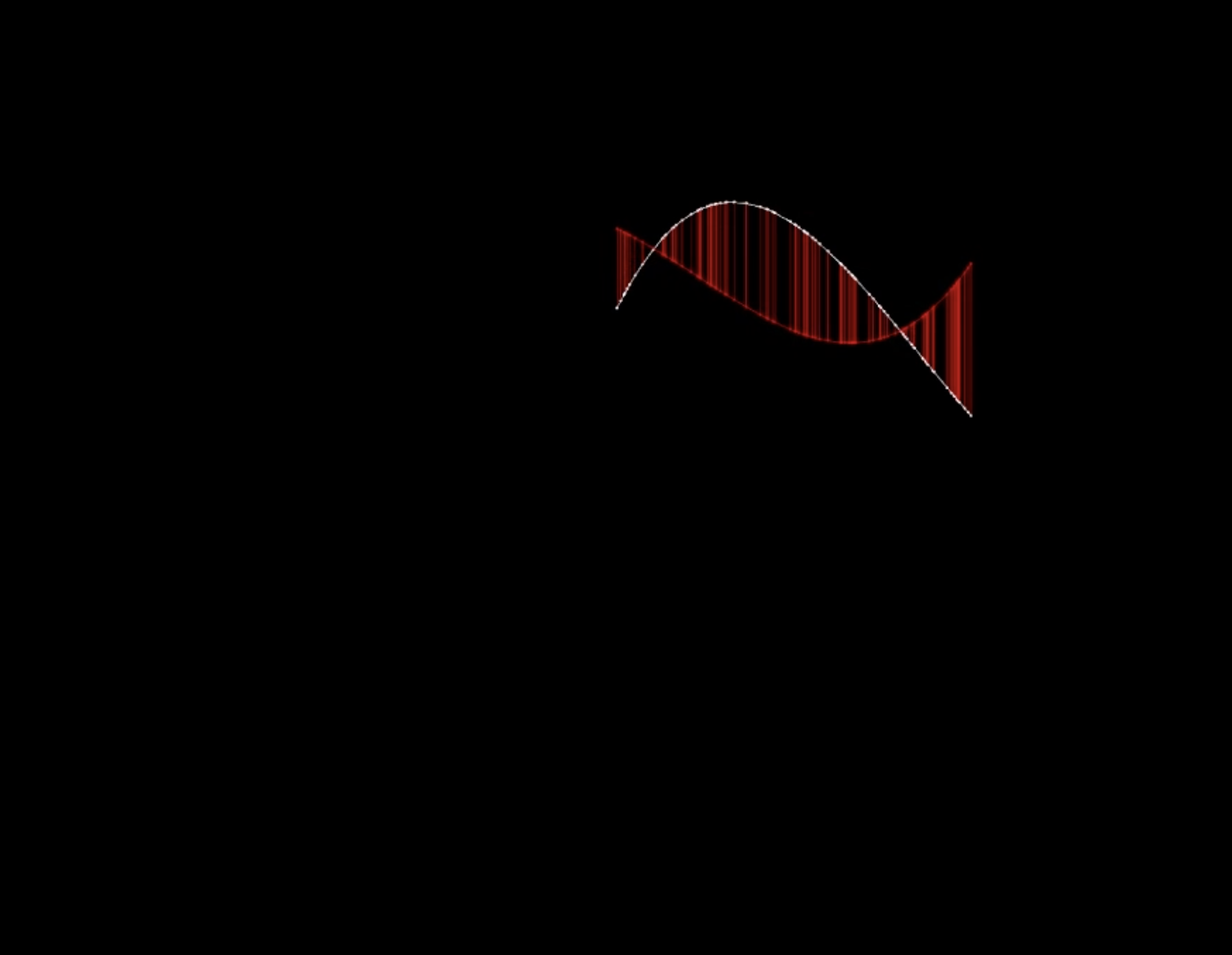
Part 1: Every time a bass note is played, a new polynomial is generated by sampling the coefficients $a,b,c,d$, and a new approximant is generated by sampling $\theta$. Every note played on the upper half of the piano induces a gradient step, and the loss of each step is used to detune the played note’s overtones. The target and learned polynomials are displayed on a black background.

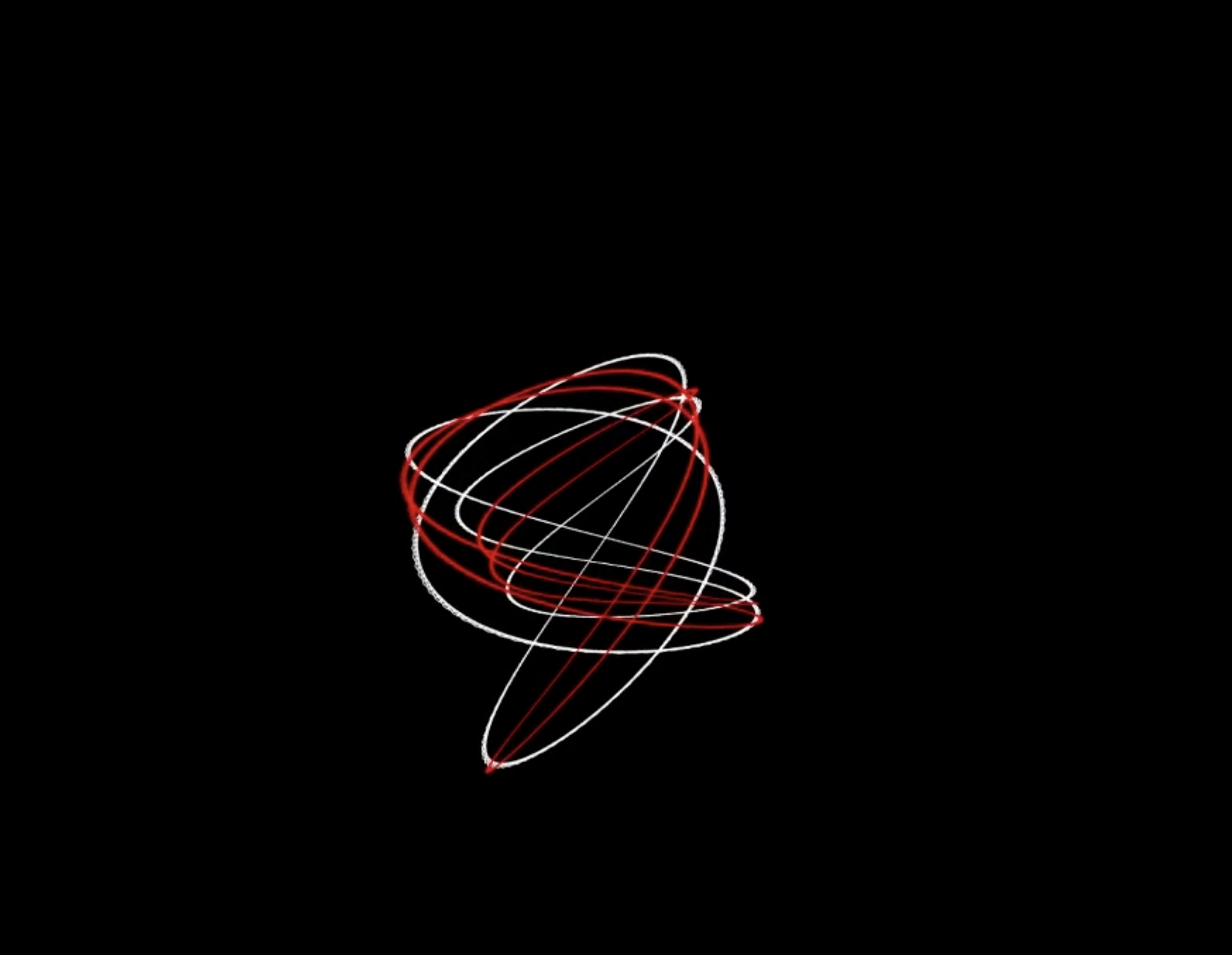
Part 2: Every time a chord is played on the left hand, a new target Lissajous knot is generated by samplinig $n_x,n_y,n_z,a,b,c$, and a new approximant is generated by sampling $\theta$. Gradient steps are continuously performed as long as the chord is held, with the loss detuning the overtones of the notes being played.

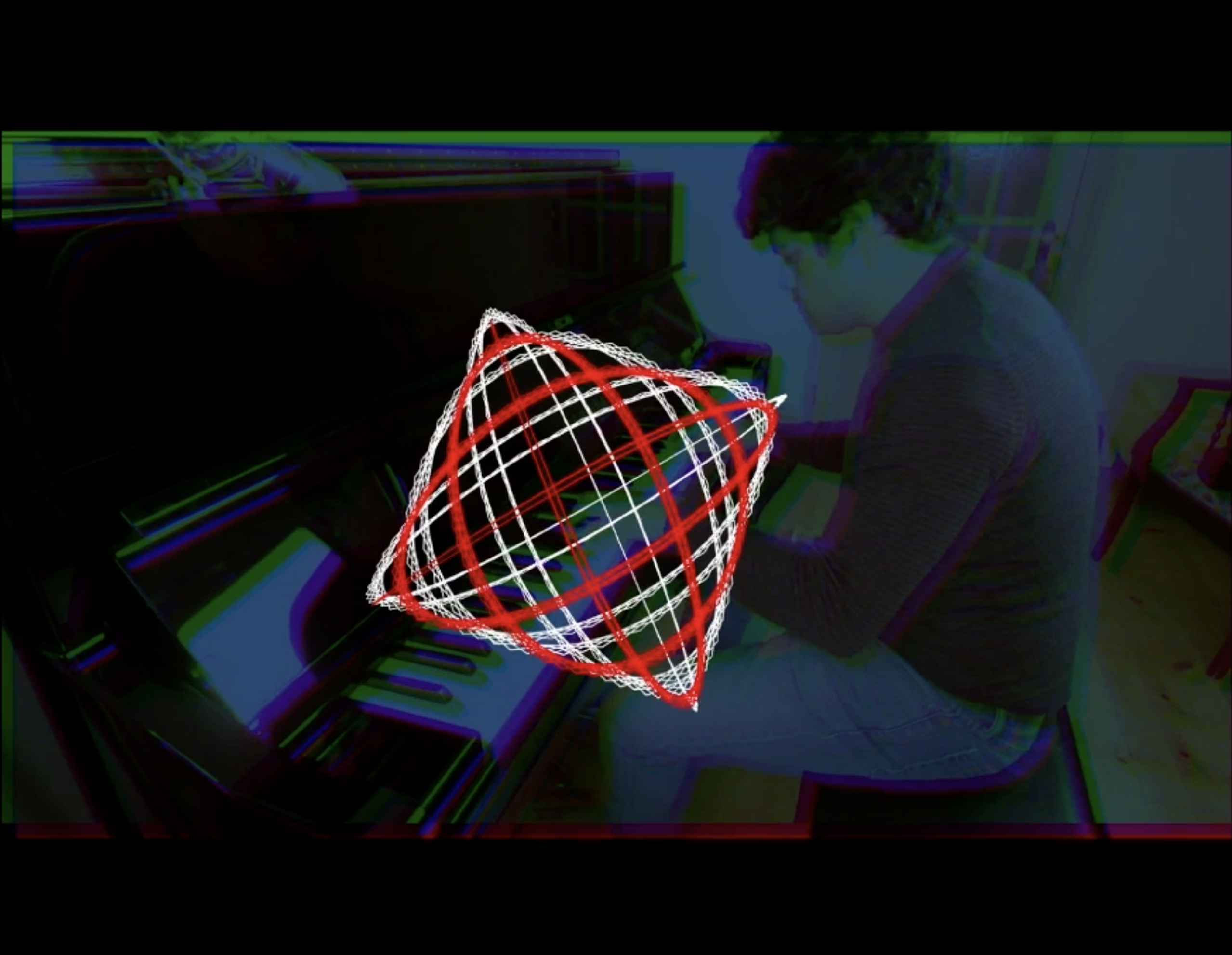
Part 3: Same as part 2, but we also display a video of the performer in the background and use Distortion (1) to affect the RGB channels.

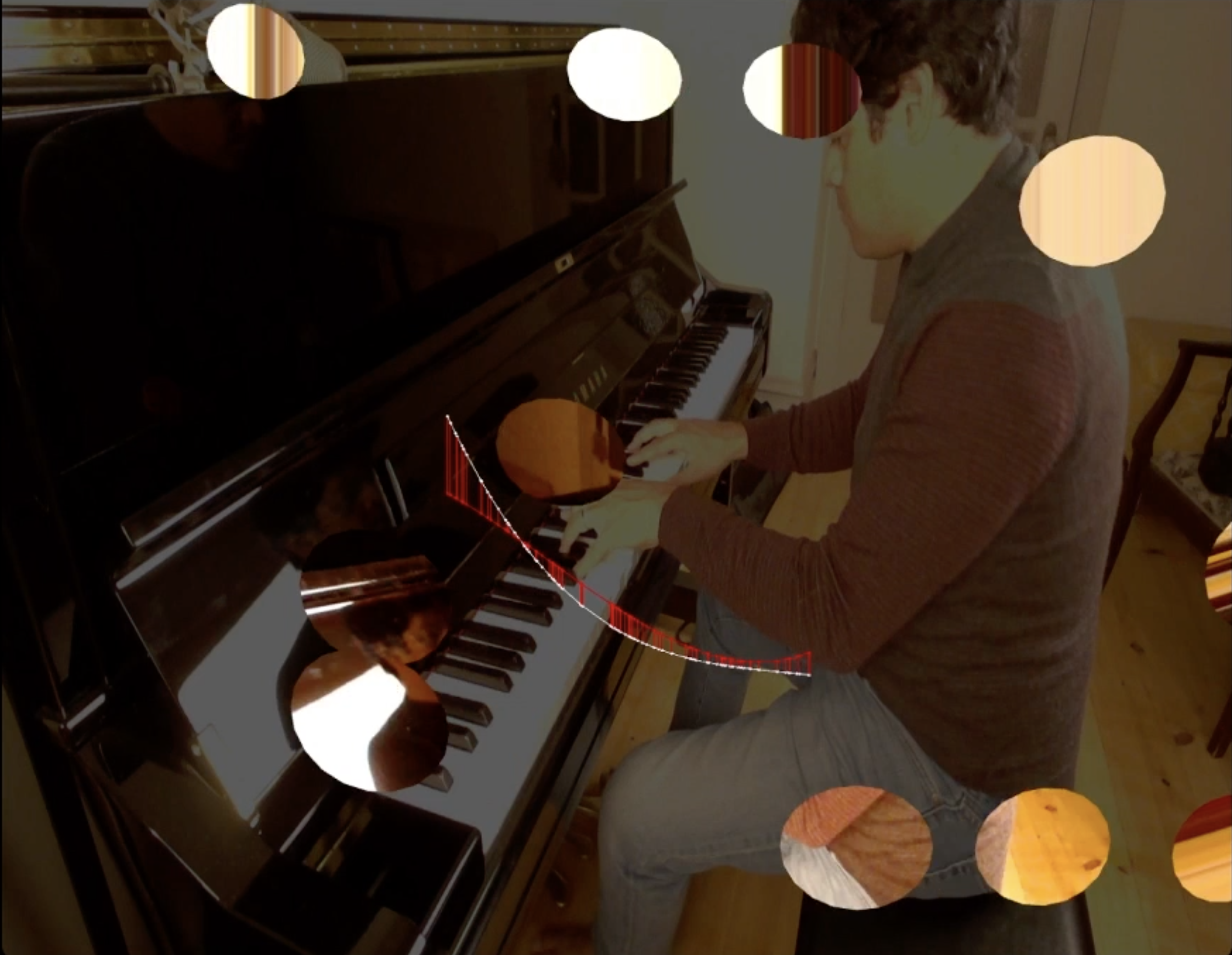
Part 4: Same as part 1, but with a video of the performer in the background. Additionally, each note played triggers a “bubble” superimposed on the video which is distorted using Distortion (2).

This is meant to be an improvised “process piece” that is different evey time it is performed.