
Pablo Samuel Castro
October 14, 2020
Introduction to reinforcement learning
This post is based on this colab.
You can also watch a video where I go through the basics here.
Pueden ver un video (en español) donde presento el material aquí.
Introduction
Reinforcement learning methods are used for sequential decision making in uncertain environments. It is typically framed as an agent (the learner) interacting with an environment which provides the agent with reinforcement (positive or negative), based on the agent’s decisions. The agent leverages this reinforcement to update its behaviour in an aim to get closer to acting optimally. In interacting with the uncertain environment, the agent is also learning about the dynamics of the underlying system.
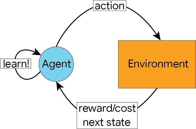
The following image depicts the typical flow of a reinforcement learning problem.
- An agent, at some state in the environment, sends an action to the environment
- The environment responds by providing the agent with:
- A reward/cost that depends on the state the agent was in and the action chosen
- A new state that the agent transitions to after performing the selected action (which can sometimes be the same state the agent was already in).
- The agent then uses this information to update its behaviour so that it increases the likelihood of choosing actions that give a positive reward, and reduces the likelihood of choosing actions that result in a penalty.
This notebook provides a brief introduction to reinforcement learning, eventually ending with an exercise to train a deep reinforcement learning agent with the dopamine framework.
The notebook is roughly organized as follows:
- A simple motivating example is presented to illustrate some of the main points and challenges.
- Markov decision processes (MDPs), the mathematical formalism used to express these problems, is introduced.
- Exact tabular methods are presented, which can be used when the environment is fully known. These methods form the foundation for the learning algorithms in uncertain environments.
- Value-based learning algorithms are introduced, and related algorithms are also presented.
- The methods introduced are put to the test on a simple MDP.
- Deep reinforcement learning is introduced, along with some implementation details.
- We use deep reinforcement learning to learn a policy on a larger MDP.
- Resources for further study are provided.
A motivating example
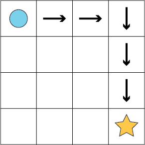
Consider the following simple grid where the agent (the blue circle) must navigate to the gold star by choosing from four actions at each grid cell (up, down, left, right):

Being able to see the whole grid, it is trivial for us to find a shortest path to the gold star (the optimal policy for the agent):
In reinforcement learning problems, however, we typically do not have immediate access to the environment. In our simple example, the agent may simply know the number of cells in the grid, but may not have any information on what is contained in each:

The agent must then explore the environment by taking actions and keeping track of what is encountered at the different cells:
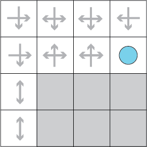
In the previous image, the grey arrows represent the actions that the agent has already taken in each of those cells. It benefits the agent to keep track of these so as to remember both the actions that lead to rewards and those that lead to penalties.
To anticipate some of the concepts that will be formalized below, the grid represents the environment. This environment consists of:
- A set of states (the grid cells)
- A set of possible actions (up, down, left, right)
- Transition dynamics, defining the effect of the actions (e.g. taking the right action will take the agent to the cell to the right of its current state)
- A reward signal that indicates the benefit or cost of the action just taken (e.g. the gold star is a positive reward received upon entering the bottom-right state).
The agent is typically aware of the states and actions, but not of the transition dynamics nor reward signal. Thus, the agent make use of a method that:
- Will explore the environment to learn about the transition and reward dynamics.
- Will keep track of previously visited states and the actions performed therein, which can be used to inform future action choices.
- Can balance exploring new experiences and exploiting the knowledge it has already achieved.
This last point is the “exploit-explore dilemma”, which is a central (and open!) problem in reinforcement learning. How to best balance this tradeoff in a computationally efficient manner is the subject of active research.
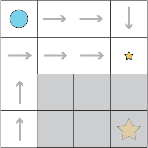
To illustrate its importance, assume the agent encountered a small reward in the grid. If at that point the agent were to decide to purely exploit its current knowledge, it would settle on the policy below, without ever exploring the unknown area where a larger reward awaits:
Having finished this motivating example, we are now ready to dive into the mathematical details.
Markov decision processes
More formally, the problem is typically expressed as a Markov decision process $\langle\mathcal{S},\mathcal{A},R,P,\gamma\rangle$, where:
- $\mathcal{S}$ is a finite set of states that the agent “inhabits”. You can also consider continuous state spaces, but for this notebook we will only be considering the finite kind.
- $\mathcal{A}$ is a finite set of actions that the agent can perform from each state. In the vast majority of cases, it is assumed that all actions are available in all states. Action spaces can also be continuous, but we will be limiting ourselves to finite action spaces in this notebook.
- $R:\mathcal{S}\times\mathcal{A}\rightarrow [R_{min}, R_{max}]\subset\mathbb{R}$ is a bounded reward (or cost) function which provides the agent with (positive or negative) reinforcement.
- $P:\mathcal{S}\times\mathcal{A}\rightarrow\Delta(\mathcal{S})$ encodes the transition dynamics, where $P(s, a)(s’)$ is the probability of ending in state $s’$ after taking action $a$ from state $s$.
- $\gamma\in[0, 1)$ is a discount factor.
The notation $\Delta(X)$ stands for the set of probability distributions over a set $X$.
Since the discount factor $\gamma$ is strictly less than $1$, it encourages the agent to accumulate rewards as quickly as possible. In the motivating example above, it means the optimal policy is also the shortest path to the big star. Having $\gamma = 1$ would mean that the agent perceives no difference between taking a short or long path to the gold star.
The agent interacts with the environment in discrete time steps. If at time step $t$ the agent is in state $s_t$ and chooses action $a_t$, the environment responds with a new state $s_{t+1}\sim P(s_t, a_t)$ and a reward $R(s_t, a_t)$.
Policies and value functions
A policy $\pi$ is a mapping from states to a distribution over actions: $\pi:\mathcal{S}\rightarrow\Delta(\mathcal{A})$, and encodes the agent’s behaviour. The value of a policy $\pi$ from an initial state $s_0$ is encoded as:
$V^{\pi}(s_0) = \left[\sum_{t=0}^{\infty}\gamma^t R(s_t, a_t) | a_t\sim\pi(s_t),s_{t+1}\sim P(s_t, a_t)\right]$
This is quantifying the expected sum of discounted rewards when starting from state $s_0$ and following policy $\pi$. It turns out we can express value functions for any state $s$ via the recurrence:
$V^{\pi}(s) = \mathbb{E}_{a\sim\pi(s)}\left[R(s, a) + \gamma\mathbb{E}_{s’\sim P(s, a)}[V^{\pi}(s’)]\right]$
or equivalently, replacing the expectation over actions with a summation:
$V^{\pi}(s) = \sum_{a\in\mathcal{A}}\pi(s)(a)\left[R(s, a) + \gamma\sum_{s’\in\mathcal{S}} P(s, a)(s’)V^{\pi}(s’)\right]$
We may sometimes also be interested in the value of performing action $a$ from state $s$, and then following policy $\pi$:
$Q^{\pi}(s, a) = R(s, a) + \gamma\mathbb{E}_{s’\sim P(s, a)}[V^{\pi}(s’)]$
Optimal policies and value functions
The goal of the agent is to find a policy $\pi^*$ that dominates all other policies: $V^* := V^{\pi^*} \geq V^{\pi}$ for all $\pi$. It turns out that there is always a deterministic policy that achieves the optimum. The Bellman optimality equations express this via the recurrence:
$V^*(s) = \max_{a\in\mathcal{A}}\left[R(s, a) + \gamma\sum_{s’\in\mathcal{S}} P(s, a)(s’)V^*(s’)\right]$
The state-action value function can be defined in a similar way as above:
$Q^*(s, a) = R(s, a) + \gamma\mathbb{E}_{s’\sim P(s, a)}[V^*(s’)]$
Clearly, we can compute $Q^*$ from $V^*$, and once we know $Q^*$ we can find $\pi^*$ via:
$\pi^*(s) = \arg\max_{a\in\mathcal{A}}Q^*(s, a)$
The important question, then, is how do we find $\pi^*$, $V^*$, and/or $Q^*$? Read on and find out!
To begin with, run the first two cells below to install and import all necessary packages.
Computing the optimal value exactly
If we have access to $P$ and $R$, then we can compute $V^*$ in a few ways. We will explore two common methods here:
- Value iteration
- Policy iteration
When the transition and reward dynamics are known, these problems are typically referred to as planning problems, which has its own field of active research. In this scenario, the “agent” does not need to interact with an environment to gather information for improving its policy. There is a close relationship between planning and reinforcement learning, and many lines of research sit at their intersection.
For our purposes, it will be useful to review some solutions to the planning problem, as they will serve as foundations for the learning algorithms we present further down.
Value iteration
In Value iteration we are continuously updating an estimate $V_{t+1}$ by leveraging our previous estimate $V_t$.
$V_{t+1}(s) := \max_{a\in\mathcal{A}} \left[ R(s, a) + \gamma \sum_{s’\in\mathcal{S}}P(s, a)(s’) V_t(s’) \right]$
This is typically referred to as the Bellman backup. It can be shown that, starting from an initial estimate $V_0$, $\lim_{t\rightarrow\infty}V_t = V^*$.
This gives us the value iteration algorithm:
- Initialize $V\equiv 0$
- Loop until convergence:
- For every $s\in\mathcal{S}$:
$V(s)\leftarrow \max_{a\in\mathcal{A}} \left[ R(s, a) + \gamma \sum_{s’\in\mathcal{S}}P(s, a)(s’) V(s’) \right]$
- For every $s\in\mathcal{S}$:
- Return $V$
It will be useful to think of the functions above as vectors, which then allows us to do the Bellman backup with matrix operations. If we assume our matrices have the following shapes:
P.shape = [num_states, num_actions, num_states]
R.shape = [num_states, num_actions]
V.shape = [num_states]
Q.shape = [num_states, num_actions]
Then we can compute $V$ with two lines of numpy code:
import numpy as np
Q = R + gamma * np.matmul(P, V)
V = np.max(Q, axis=1)
Alternatively, we can use the einsum function, which can help clarify the dimensions along which the multiplication is happening:
Q = R + gamma * np.einsum('sat,t->sa', P, V)
V = np.max(Q, axis=1)
As mentioned above, once we have $V^*$, we can compute $Q^*$ and $\pi^*$.
The code cell below is an implementation of value iteration.
def value_iteration(P, R, gamma, tolerance=1e-3):
  """Find V* using value iteration.

  Args:
    P: numpy array defining transition dynamics. Shape: |S| x |A| x |S|.
    R: numpy array defining rewards. Shape: |S| x |A|.
    gamma: float, discount factor.
    tolerance: float, tolerance level for computation.

  Returns:
    V*: numpy array of shape ns.
    Q*: numpy array of shape ns x na.
  """
  assert P.shape[0] == P.shape[2]
  assert P.shape[0] == R.shape[0]
  assert P.shape[1] == R.shape[1]
  ns = P.shape[0]
  na = P.shape[1]
  V = onp.zeros(ns)
  Q = onp.zeros((ns, na))
  error = tolerance * 2
  while error > tolerance:
    # This is the Bellman backup (onp.einsum FTW!).
    Q = R + gamma * onp.einsum('sat,t->sa', P, V)
    new_V = onp.max(Q, axis=1)
    error = onp.max(onp.abs(V - new_V))
    V = onp.copy(new_V)
  return V, Q
Policy iteration
Instead of iterating over $V_t$, we can iterate over $\pi_t$ and stop once the policy is no longer changing. The algorithm proceeds as follows:
- Initialize $\pi$ arbitrarily. For simplicity we will assume it is a matrix of shape
[num_states, num_actions]with only one1.0for each row (i.e. a deterministic policy). - While $\pi$ is changing:
- $Q(s, a) = R(s, a) + \gamma\sum_{s’\in\mathcal{S}}P(s, a)(s’)Q(s’, \pi(s’))$
- $\pi(s) = \arg\max Q(s, \cdot)$
- $Q(s, a) = R(s, a) + \gamma\sum_{s’\in\mathcal{S}}P(s, a)(s’)Q(s’, \pi(s’))$
- $V(s) = \max_{a\in\mathcal{A}}Q(s, a)$
- Return $V$
Notice that, in contrast to value iteration, here we compute $Q^*$ and $V^*$ from $\pi^*$.
def policy_iteration(P, R, gamma):
  """Find V* using policy iteration.

  Args:
    P: numpy array defining transition dynamics. Shape: |S| x |A| x |S|.
    R: numpy array defining rewards. Shape: |S| x |A|.
    gamma: float, discount factor.

  Returns:
    V*: numpy array of shape ns.
    Q*: numpy array of shape ns x na.
  """
  assert P.shape[0] == P.shape[2]
  assert P.shape[0] == R.shape[0]
  assert P.shape[1] == R.shape[1]
  ns = P.shape[0]
  na = P.shape[1]
  V = onp.zeros(ns)
  Q = onp.zeros((ns, na))
  pi = onp.zeros((ns, na))
  for s in range(ns):
    pi[s, onp.random.choice(na)] = 1.
  policy_stable = False
  while not policy_stable:
    old_pi = onp.copy(pi)
    # Extract V from Q using pi.
    V = [Q[s, onp.argmax(pi[s])] for s in range(ns)]
    Q = R + gamma * onp.einsum('sat,t->sa', P, V)
    pi = onp.zeros((ns, na))
    for s in range(ns):
      pi[s, onp.argmax(Q[s])] = 1.
    policy_stable = onp.array_equal(pi, old_pi)
  V = [Q[s, onp.argmax(pi[s])] for s in range(ns)]
  Q = R + gamma * onp.einsum('sat,t->sa', P, V)
  V = [Q[s, onp.argmax(pi[s])] for s in range(ns)]
  return V, Q
Learning the optimal value
What if one does not have access to $P$ and $R$? This is the most common scenario in reinforcement learning problems, and here the agents must learn how to behave by interacting with the environment.
The diagram below depicts this pictorially:
- The agent, in state $s$, picks an action $a$ from its policy $\pi(s)$ and sends this action to the environment.
- The environment returns a new state $s’\sim P(s, a)$ and reward $R(s, a)$ to the agent.
- The agent can then use this new information to update its policy $\pi$.
Model-based versus model-free approaches
Two common approaches for handling this are:
- Model-based methods: Learn approximate models $\hat{P}$ and $\hat{R}$ from the experience received from the environment, and solve for $\hat{V}^*$, $\hat{Q}^*$, and $\hat{\pi}^*$ using value/policy iteration.
- Model-free methods: Learn approximates $\hat{V}^*$, $\hat{Q}^*$, and/or $\hat{\pi}^*$ using the experience received from the environment.
There are pros and cons for each of these approaches, and there is extensive (and continuing) research for both.
For example, model-based methods tend to be more sample-efficient, since one can always sample from $\hat{P}$ and $\hat{R}$ without having to interact with the real environment.
On the other hand, model-free methods are typically easier to learn and update in an online fashion (as new experience arrives), which is usually desirable.
Value-based versus policy-based approaches
Within model-free methods, there are two main approaches used: value-based versus policy-based.
- Value-based methods maintain and update an estimate for $Q^*$
- Policy-based methods maintain and update an estimate for $\pi^*$
Once again, there are pros and cons and extensive literature for both of these approaches.
In this notebook, we will focus on value-based methods.
You can learn more about policy-based methods in the Sutton & Barto book and in the Spinning up in Deep RL post by Open-AI.
Exploration
One of the central issues in reinforcement learning is the exploration-exploitation dilemma. This was briefly introduced in the motivating example at the top, but is critical to the eventual performance of the agent.
Consider an agent that started with an initial policy $\pi_0$, and at iteration $t$ has policy $\pi_t$ and state-action value function $Q^{\pi_t}\gg Q^{\pi_0}$. While at state $s$, the natural thing would be for the agent to pick action $a = \pi_t(s) = \arg\max_{a\in\mathcal{A}}Q^{\pi_t}(s, a)$. This would be a purely exploitative policy.
What if, had the agent picked a different action, $b\ne a$ that resulted in a very large reward? Imagine the agent had selected action $b$ and the new estimate $Q_{t+1}$ had the property that $Q_{t+1}(s, b) > Q_{t+1}(s, a)$, then the policy would be updated as $\pi_{t+1}(s) = b$.
At iteration $t$, by definition, $Q^{\pi_t}(s, b) < Q^{\pi_t}(s, a)$, so the agent would have never selected action $b$ with a purely exploitative policy, thereby missing out on a larger reward! Thus, it would have benefited the agent to select sub-optimal action $b$ to uncover the larger reward.
Selecting a sub-optimal action is what is referred to as exploration, since the reasoning behind choosing sub-optimally is precisely to explore the environment and potentially discover better policies.
A purely exploratory policy would not be desirable either, as the agent would then always select actions randomly, which would make it unlikely to maximize the expected rewards received.
As mentioned previously, balancing this exploration-exploitation tradeoff is a very active area of research.
$\epsilon$-greedy exploration
Perhaps the simplest and best-known exploration method is $\epsilon$-greedy exploration. At state $s$, given a policy $\pi$, the rule for this exploration policy is simply:
- With probability $\epsilon$ select an action randomly
- With probability $1-\epsilon$ select action $a=\arg\max_{a\in\mathcal{A}}\pi(s)$
The code snippet below implements this exploratory policy.
def epsilon_greedy(s, pi, epsilon):
  """A simple implementation of epsilon-greedy exploration.

  Args:
    s: int, the agent's current state.
    pi: numpy array of shape [num_states, num_actions] encoding the agent's
      policy.
    epsilon: float, the epsilon value for epsilon-greedy exploration.

  Returns:
    An integer representing the action choice.
  """
  na = pi.shape[1]
  p = onp.random.rand()
  if onp.random.rand() < epsilon:
    return onp.random.choice(na)
  return onp.random.choice(na, p=pi[s])
Monte Carlo methods
Perhaps the simplest way of estimating the sum of future returns is using Monte Carlo methods. These methods execute full trajectories in the environment and estimate $V^{\pi}$ by averaging the observed trajectory returns.
The algorithm can be described as follows:
- Initialize $Q$ and pick a start state $s$.
- Initialize a list $Returns$ of $|\mathcal{S}|\times|\mathcal{A}|$ elements which accumulates observed returns for each state.
- Initialize $\pi$ randomly.
- While learning:
- Generate a trajectory $\langle s_0,a_0,r_0,\cdots,s_T,a_T,r_T\rangle$ using $\pi$.
- $G = 0$
- For $t=T$ down to $0$:
- $G = \gamma G + r_t$
- If $(s_t,a_t)$ does not appear in $\langle s_0,a_0,\cdots,s_{t-1},a_{t-1}\rangle$:
- Append $G$ to $Returns(s_t, a_t)$
- $Q(s_t, a_t) = average(Returns(s_t, a_t))$
- $\pi(s_t) = \arg\max_{a\in\mathcal{A}} Q(s_t, a)$
The next code cell implements this approach.
def monte_carlo(ns, na, step_fn, gamma, start_state, reset_state, total_episodes,
               max_steps_per_iteration, epsilon, V):
  """A simple implementation of Q-learning.

  Args:
    ns: int, the number of states.
    na: int, the number of actions.
    step_fn: a function that receives a state and action, and returns a float
      (reward) and next state. This represents the interaction with the
      environment.
    gamma: float, the discount factor.
    start_state: int, index of starting state.
    reset_state: int, index of state where environment resets back to start
      state, or None if there is no reset state.
    total_episodes: int, total number of episodes.
    max_steps_per_iteration: int, maximum number of steps per iteration.
    epsilon: float, exploration rate for epsilon-greedy exploration.
    V: numpy array, true V* used for computing errors. Shape: [num_states].

  Returns:
    V_hat: numpy array, learned value function. Shape: [num_states].
    Q_hat: numpy array, learned Q function. Shape: [num_states, num_actions].
    max_errors: list of floats, contains the error max_s |V*(s) - \hat{V}*(s)|.
    avg_errors: list of floats, contains the error avg_s |V*(s) - \hat{V}*(s)|.
  """
  # Initialize policy randomly.
  pi_hat = onp.zeros((ns, na))
  for s in range(ns):
    pi_hat[s, onp.random.choice(na)] = 1.
  # Initialize Q randomly.
  Q_hat = onp.zeros((ns, na))
  # Initialize the accumulated returns and number of updates.
  returns = onp.zeros((ns, na))
  counts = onp.zeros((ns, na))
  # Lists to keep track of training statistics.
  iteration_returns = []
  max_errors = []
  avg_errors = []
  for episode in range(total_episodes):
    # Each episode starts in the same start state.
    s = start_state
    step = 0
    # Lists collected for each trajectory.
    states = []
    actions = []
    rewards = []
    # Generate a trajectory for a limited number of steps.
    while step < max_steps_per_iteration:
      step += 1
      states.append(s)
      a = epsilon_greedy(s, pi_hat, epsilon)  # Pick action.
      actions.append(a)
      r, s2 = step_fn(s, a)  # Take a step in the environment.
      rewards.append(r)
      if s2 == reset_state:
        # If we've reached a reset state, the trajectory is over.
        break
      s = s2
    # Update the Q-values based on the rewards received by traversing the
    # trajectory in reverse order.
    G = 0  # Accumulated returns.
    step -= 1
    while step >= 0:
      G = gamma * G + rewards[-1]
      rewards = rewards[:-1]
      s = states[-1]
      states = states[:-1]
      a = actions[-1]
      actions = actions[:-1]
      # We only update Q(s, a) for the first occurence of the pair in the
      # trajectory.
      update_q = True
      for i in range(len(states)):
        if s == states[i] and a == actions[i]:
          update_q = False
          break
      if update_q:
        returns[s, a] += G
        counts[s, a] += 1
        Q_hat[s, a] = returns[s, a] / counts[s, a]
        pi_hat[s] = onp.zeros(na)
        pi_hat[s, onp.argmax(Q_hat[s])] = 1.
      step -= 1
    iteration_returns.append(G)
    V_hat = onp.max(Q_hat, axis=1)
    max_errors.append(onp.max(onp.abs(V - V_hat)))
    avg_errors.append(onp.mean(onp.abs(V - V_hat)))
  return V_hat, Q_hat, iteration_returns, max_errors, avg_errors
Q-learning
Although Monte Carlo methods can update value estimates based on interactions with the environment, a more common approach in reinforcement learning is to use Temporal-Difference (TD) methods. This approach combines ideas from Monte Carlo estimation and dynamic programming.
Like Monte Carlo methods, Q-learning updates its estimates from sampled experiences; but like dynamic programming methods, it does so with single-step transitions. In its simplest form, after performing action $a$ from state $s$ and observing reward $r$ and next state$s’$, Q-learning updates its estimate of $V^{\pi}(s)$ as follows:
$Q^{\pi}(s, a) = V^{\pi}(s) + \alpha\left[ r + \gamma V^{\pi}(s’) - V^{\pi}(s)\right]$
Here, $\alpha\in[0, 1]$ is the step size, and determines how aggressively we will update our estimates given new evidence from the environment.
In this simplified setting we are assuming $\alpha$ remains fixed once selected, but there are more sophisticated methods which varies it throughout training. The algorithm proceeds as follows:
- Initialize $Q$ and $\pi$, and pick a start state $s$.
- While learning:
- Pick action $a$ according to $\pi$ (and any exploratory policy).
- Send $a$ to the environment and receive $s’$ and $r$ in return.
- Compute the TD-error as:
$\delta = r + \gamma \max_{a’\in\mathcal{A}}Q(s’, a’) - Q(s, a)$ - Update the estimate for $Q(s, a)$ as follows:
$Q(s, a) = Q(s, a) + \alpha\delta$ - $\pi(s) = \arg\max_{a\in\mathcal{A}} Q(s, a)$
- Update $s = s’$.
The next cell provides an implementation of Q-learning.
def q_learning(ns, na, step_fn, gamma, start_state, reset_state, total_episodes,
               max_steps_per_iteration, epsilon, alpha, V):
  """A simple implementation of Q-learning.

  Args:
    ns: int, the number of states.
    na: int, the number of actions.
    step_fn: a function that receives a state and action, and returns a float
      (reward) and next state. This represents the interaction with the
      environment.
    gamma: float, the discount factor.
    start_state: int, index of starting state.
    reset_state: int, index of state where environment resets back to start
      state, or None if there is no reset state.
    total_episodes: int, total number of episodes.
    max_steps_per_iteration: int, maximum number of steps per iteration.
    epsilon: float, exploration rate.
    alpha: float, learning rate.
    V: numpy array, true V* used for computing errors. Shape: [num_states].

  Returns:
    V_hat: numpy array, learned value function. Shape: [num_states].
    Q_hat: numpy array, learned Q function. Shape: [num_states, num_actions].
    max_errors: list of floats, contains the error max_s |V*(s) - \hat{V}*(s)|.
    avg_errors: list of floats, contains the error avg_s |V*(s) - \hat{V}*(s)|.
  """
  # Initialize policy randomly.
  pi_hat = onp.zeros((ns, na))
  for s in range(ns):
    pi_hat[s, onp.random.choice(na)] = 1.
  # Initialize Q to zeros.
  Q_hat = onp.zeros((ns, na))
  # Lists collected for each trajectory.
  iteration_returns = []
  max_errors = []
  avg_errors = []
  for episode in range(total_episodes):
    # Each episode begins in the same start state.
    s = start_state
    step = 0
    num_episodes = 0
    steps_in_episode = 0
    cumulative_return = 0.
    average_episode_returns = 0.
    # Interact with the environment for a maximum number of steps
    while step < max_steps_per_iteration:
      a = epsilon_greedy(s, pi_hat, epsilon)  # Pick action.
      r, s2 = step_fn(s, a)  # Take a step in the environment.
      delta = r + gamma * max(Q_hat[s2]) - Q_hat[s, a]  # TD-error.
      Q_hat[s, a] += alpha * delta  # Q-learning update.
      cumulative_return += gamma**(steps_in_episode) * r
      pi_hat[s] = onp.zeros(na)
      pi_hat[s, onp.argmax(Q_hat[s])] = 1.
      s = s2
      steps_in_episode += 1
      if s2 == reset_state:
        s = 0
        num_episodes += 1
        steps_in_episode = 0
        average_episode_returns += cumulative_return
        cumulative_return = 0.
      step += 1
    average_episode_returns /= max(1, num_episodes)
    iteration_returns.append(average_episode_returns)
    V_hat = onp.max(Q_hat, axis=1)
    max_errors.append(onp.max(onp.abs(V - V_hat)))
    avg_errors.append(onp.mean(onp.abs(V - V_hat)))
  return V_hat, Q_hat, iteration_returns, max_errors, avg_errors
Colab!
The rest of this intro is hands-on, so you should follow the instructions in the colab.
comments powered by Disqus